Principal Component Analysis (PCA)

17. Principal Component Analysis (PCA)#

Principal Component Analysis (PCA) is a powerful unsupervised learning method used for finding the axes of maximum variation in your data and projecting the data into new coordinate systems.

17.1. Decomposition of a matrix#

From linear algebra, we know that we can multiply two vectors into a matrix. $$ \mathbf{X} = \mathbf{u} \otimes \mathbf{v} = \mathbf{u} \mathbf{v}^{\textsf{T}} = \begin{bmatrix} u_1 \\ u_2 \\ u_3 \\ u_4 \end{bmatrix} \begin{bmatrix} v_1 & v_2 & v_3 \end{bmatrix} = \begin{bmatrix} u_1 v_1 & u_1 v_2 & u_1 v_3 \\ u_2 v_1 & u_2 v_2 & u_2 v_3 \\ u_3 v_1 & u_3 v_2 & u_3 v_3 \\ u_4 v_1 & u_4 v_2 & u_4 v_3 \end{bmatrix}. $$
What if we could do the opposite? I.e., given a matrix $\mathbf{X}$, what would be the vectors $\mathbf{u}$ and $\mathbf{v}$ that best represent $\mathbf{X}$ so that $\mathbf{X} \approx \mathbf{u} \mathbf{v}^{\textsf{T}}$? This is, in essence, what you do with principal component analysis (PCA).

17.1.1. A scenario where this might be useful#

In PCA, we often deal with a matrix that encapsulates multiple sources of variation. Imagine a scenario where we’re studying gene expression levels across several samples. Here, the gene expression levels might be influenced by two key factors:

Gene-Specific Effects: These are inherent to each gene, such as its baseline expression level or potential for expression. For example, some genes may generally be expressed at high levels across all conditions, while others have lower baseline expression.
Sample-Specific Effects: These capture the influence of each sample (environmental condition, patient, disease state) on gene expression. For instance, one condition might increase expression levels across many genes, while another has a weaker or even suppressive effect.

By setting up the gene expression matrix $X$ as a product of two vectors:

\[X = u \cdot v^T\]

we express the matrix as an outer product of these two effects:

$u$ represents the gene-specific effects.
$v$ represents the sample-specific effects.

When we perform PCA on $ X $, the primary principal component should capture the main pattern driven by these combined effects, showing a dominant structure that reflects how genes and samples contribute to variation together. Secondary components may capture additional variations or deviations, if any, from this main trend.

17.1.2. Fictive Example#

Now, let’s apply this theory in a concrete, 4x4 example with 4 samples and 4 genes. Here, we will see how gene-specific and sample-specific effects can combine to form the observed matrix.

17.1.2.1. Setup#

Let:

$u$ be a vector representing the gene-specific effects: $ u = [2, 1, 0.5, 3] $.
$v$ be a vector representing the sample-specific effects: $ v = [1, 0.8, 1.2, 0.5] $.

To build our matrix $ X $, we calculate the outer product $ X = u \cdot v^T $, where each entry $ X_{ij} = u_i \cdot v_j $.

17.1.2.2. Calculations#

Gene-Specific Effects $ u = [2, 1, 0.5, 3] $
Sample-Specific Effects $ v = [1, 0.8, 1.2, 0.5] $

Using the outer product:

\[\begin{split} X = \begin{bmatrix} 2 \\ 1 \\ 0.5 \\ 3 \end{bmatrix} \cdot \begin{bmatrix} 1 & 0.8 & 1.2 & 0.5 \end{bmatrix} = \begin{bmatrix} 2 & 1.6 & 2.4 & 1 \\ 1 & 0.8 & 1.2 & 0.5 \\ 0.5 & 0.4 & 0.6 & 0.25 \\ 3 & 2.4 & 3.6 & 1.5 \end{bmatrix} \end{split}\]

17.1.2.3. Interpretation#

In practice, we usually start with the observed matrix $ X $—for example, the gene expression levels across samples. The goal of PCA is to approximate this observed matrix by finding underlying factors (similar to $u$ and $v$ in this example) that explain the main sources of variation. In this fictive example, the matrix $ X $ is constructed directly from $u$ and $v$, representing gene-specific and sample-specific effects.

If we only had access to $ X $, PCA would allow us to decompose it into components that reflect these underlying patterns of variation. The first principal component would likely capture the dominant trend influenced by both gene-specific and sample-specific effects, while subsequent components might explain additional variability not captured by the primary trend.

This example helps to understand that, through PCA, we are essentially trying to express the observed data as a combination of simpler underlying factors, much like how $ X $ here is represented as an outer product of $u$ and $v$.

17.1.3. Scaling the components#

When decomposing a matrix with PCA, we aim to find directions that capture the main sources of variation. For a matrix $ X $, where we assume a factorization as an outer product of two vectors $ u $ and $ v $, the decomposition can be represented as:

\[ X \approx S \cdot u \cdot v^T \]

where $ S $ is a scalar that captures the magnitude, while $ u $ and $ v $ provide the directions.

In PCA, the directions $ u $ and $ v $ indicate the axes along which most of the data’s variance lies. However, the magnitude of the variation (how much variance is explained) can technically be distributed between $ u $ and $ v $. This is because if we scale $ u $ by a factor $ \alpha $ and scale $ v $ by $ 1 / \alpha $, the product $ u \cdot v^T $ remains the same, allowing flexibility in how we allocate the magnitude.

To standardize this decomposition, it is common to select $ u $ and $ v $ to have a norm of 1. This normalization ensures that $ u $ and $ v $ only represent directions, while the entire magnitude of the variation is captured by the scalar $ s $. Thus, $ s $ becomes a single value that encapsulates the strength of the variation along the principal component, while $ u $ and $ v $ are pure directional vectors, each constrained to unit length:

\[ \| u \| = 1, \quad \| v \| = 1 \]

This approach makes the interpretation of the PCA decomposition more consistent, as $ s $ represents the variance captured by this component, and $ u $ and $ v $ describe the specific directions of variation in row and column space, respectively.

17.2. More principal components to your PCA#

Once you remove the principal components from a matrix $\mathbf{X}$, the remaining residues, i.e., $\mathbf{X - S_1u^{(1)} v^{(1)T}}$, might in turn be decomposed into vectors. We can calculate the vectors $\mathbf{u^{(2)}}$ and $\mathbf{v^{(2)}}$ that best describe the matrix $\mathbf{X - S_1u^{(1)} v^{(1)T}}$. These are called the second principal components, while the original ones are called the first principal components.
In this manner, we can derive as many principal components as there are rows or columns (whichever is smaller) in $\mathbf{X}$. In most applications, we settle for two such components.

17.3. An illustration of PCA#

	Sample $1$	Sample $2$	Sample $3$		Sample $M$	Gene specific $\mathbf{u}^{(1)}$	Gene specific $\mathbf{u}^{(2)}$
Gene $1$	$X_{11}$	$X_{12}$	$X_{13}$	$\ldots$	$X_{1M}$	$u^{(1)}_1$	$u^{(2)}_1$
Gene $2$	$X_{21}$	$X_{22}$	$X_{23}$	$\ldots$	$X_{2M}$	$u^{(1)}_2$	$u^{(2)}_2$
Gene $3$	$X_{31}$	$X_{32}$	$X_{33}$	$\ldots$	$X_{3M}$	$u^{(1)}_3$	$u^{(2)}_3$
$\vdots$	$\vdots$	$\vdots$	$\vdots$	$\ddots$	$\vdots$	$\vdots$	$\vdots$
Gene $N$	$X_{N1}$	$X_{N2}$	$X_{N3}$	$\ldots$	$X_{NM}$	$u^{(1)}_N$	$u^{(2)}_N$

Sample specific $\mathbf{v}^{T(1)}$	$v^{(1)}_1$	$v^{(1)}_2$	$v^{(1)}_3$	$\ldots$	$v^{(1)}_M$	$S_1$
Sample specific $\mathbf{v}^{T(2)}$	$v^{(2)}_1$	$v^{(2)}_2$	$v^{(2)}_3$	$\ldots$	$v^{(2)}_M$		$S_2$

17.4. Principal Components#

PCA aims to identify the directions, or principal components, in the data that describe the most variance. These directions are essentially the new axes into which the original data is projected, and they help us gain insight into the underlying structure and patterns. The principal components are ordered such that the first principal component describes the largest possible variance, while each subsequent component describes as much of the remaining variance as possible, subject to being orthogonal to the preceding components.

An interesting property of PCA is that the principal components derived from a data matrix $ X $ are equivalent to the projections of the principal components derived from the transposed matrix $ X^T $. In our example, the gene-specific effects ($u$) and the sample-specific effects ($v$) can be thought of as such principal component pairs. Each pair of principal components, derived from both rows and columns of the matrix, helps to minimize the squared sum of residuals, providing an optimal lower-dimensional representation of the data. This means that the decomposition we see with $u$ and $v$ is similar to what PCA aims to achieve: capturing the most significant variation in the data through paired components.

Suppose we have a data matrix $X$, and we are focusing on just the first pair of principal components, If you project $X$ onto $v^{(1)}$, you are essentially collapsing the information in each row of $X$ along the direction of the first principal component represented by $v^{(1)}$. This gives you a score for each row of $X$, which can be seen as the projection of $X$ on $v^{(1)}$. Similarly, if you project $X^T$ onto $u^{(1)}$, you are collapsing the information in each column of $X$ along the direction of the first principal component represented by $u^{(1)}$. This gives you a score for each column of $X$, $v^{(1)}$, also scaled by the singular value $S_1$.

Thus, we can say:

$u^{(1)}$ is what you get (up to a scaling factor) when you project $X$ on $v^{(1)}$.
$v^{(1)}$ is what you get (up to a scaling factor) when you project $X^T$ on $u^{(1)}$.

17.5. Dimensionality Reduction and Explained Variance#

One of the key advantages of PCA is dimensionality reduction. By focusing only on the principal components that describe most of the variance in the data, PCA allows us to reduce the number of random variables under consideration. This is particularly useful when dealing with high-dimensional datasets, such as those encountered in genomics and transcriptomics, where the number of features (e.g., genes) can be overwhelming.

The contribution of each principal component to the overall variance is called the explained variance. The first principal component typically explains the most variance, followed by the second, and so on. By examining the explained variance, we can determine how many principal components are needed to capture most of the important variation in the data. For instance, if the first few principal components explain a large proportion of the total variance, then the dimensionality of the dataset can be substantially reduced without significant loss of information.

17.6. Singular Value Decomposition (SVD)#

The calculation of principal components can be efficiently performed using singular value decomposition (SVD), a fundamental linear algebra technique. Given a data matrix $X$, SVD decomposes it as follows:

\[X = USV^T\]

Here:

$U$ is a matrix formed from the Gene-Specific Effects.
$V^T$ is a matrix formed from the Sample-Specific Effects.
$S$ is a diagonal matrix that carries the magnitude (singular values) of each principal component pair.

SVD provides a robust way to perform PCA, allowing for the identification of eigensamples and eigengenes while efficiently capturing the major patterns in the data. Since $S$ contains the singular values, it directly relates to the explained variance of the principal components, with larger singular values corresponding to more significant components.

A practical use of the singular values is that they give the amount of variance explained by each principal component. Typically we are interested in computing the percentage of variance explained by component $i$ as $R^2_i=\frac{s^2_i}{\sum_j s^2_j}$.

17.7. Affine Transformation and Interpretation#

PCA is an affine transformation, meaning that it can involve translation, rotation, and uniform scaling of the original data. Importantly, PCA maintains the relationships between points, straight lines, and planes, which allows for a meaningful geometric interpretation of the results. By transforming the data into a new set of axes aligned with the directions of maximum variance, PCA enables us to discover the key structural relationships while preserving important properties.

17.8. Applications of PCA#

In data science, PCA is widely applied for visualization, clustering, and feature extraction. In biotechnology, PCA is often used to:

Identify major sources of variation in gene expression data.
Visualize sample relationships in a reduced-dimensional space.
Detect batch effects and outliers in high-throughput experiments.

By applying PCA, researchers can distill complex, high-dimensional data into a manageable form, making it easier to interpret and analyze the underlying biological phenomena.

17.9. An example of reconstruction with PCA, Eigenfaces#

import matplotlib.pyplot as plt
from numpy.random import RandomState

from sklearn import cluster, decomposition
from sklearn.datasets import fetch_olivetti_faces
from sklearn.decomposition import PCA

rng = RandomState(0)


# Load the Olivetti faces dataset
faces, _ = fetch_olivetti_faces(return_X_y=True, shuffle=True, random_state=rng)
n_samples, n_features = faces.shape

# Global centering (focus on one feature, centering all samples)
faces_centered = faces - faces.mean(axis=0)

# Local centering (focus on one sample, centering all features)
faces_centered -= faces_centered.mean(axis=1).reshape(n_samples, -1)

print("Dataset consists of %d faces" % n_samples)

# Define a base function to plot the gallery of faces
n_row, n_col = 5, 4
n_components = n_row * n_col
image_shape = (64, 64)

def plot_gallery(title, images, n_col=n_col, n_row=n_row, cmap=plt.cm.gray):
    fig, axs = plt.subplots(
        nrows=n_row,
        ncols=n_col,
        figsize=(2.0 * n_col, 2.3 * n_row),
        facecolor="white",
        constrained_layout=True,
    )
    fig.set_constrained_layout_pads(w_pad=0.01, h_pad=0.02, hspace=0, wspace=0)
    fig.set_edgecolor("black")
    fig.suptitle(title, size=16)
    for ax, vec in zip(axs.flat, images):
        vmax = max(vec.max(), -vec.min())
        im = ax.imshow(
            vec.reshape(image_shape),
            cmap=cmap,
            interpolation="nearest",
            vmin=-vmax,
            vmax=vmax,
        )
        ax.axis("off")

    fig.colorbar(im, ax=axs, orientation="horizontal", shrink=0.99, aspect=40, pad=0.01)
    plt.show()

# Create a PCA model and fit it to the centered faces
print("Fitting PCA model to faces dataset...")
pca = PCA(n_components=n_components, whiten=True, random_state=rng)
pca.fit(faces_centered)

# Extract the eigenfaces (principal components)
eigenfaces = pca.components_

# Plot the first n_components eigenfaces
plot_gallery("Eigenfaces (Principal Components)", eigenfaces[:n_components])

# Project the original faces onto the PCA components to get their low-dimensional representation
faces_pca_projection = pca.transform(faces_centered)

# Reconstruct the faces using the PCA projection
faces_reconstructed = pca.inverse_transform(faces_pca_projection)

# Plot a gallery of original and reconstructed faces for comparison
plot_gallery("Original Centered Faces", faces_centered[:4*5],5,4)
plot_gallery("Reconstructed Faces", faces_reconstructed[:4*5],5,4)

print("Explained variance ratio of components: ", pca.explained_variance_ratio_)

# Optional: Show how much variance is explained by the components
plt.figure(figsize=(8, 5))
plt.plot(range(1, n_components + 1), pca.explained_variance_ratio_, marker='o', linestyle='--')
plt.xlabel('Principal Component Index')
plt.ylabel('Explained Variance Ratio')
plt.title('Explained Variance by Each Principal Component')
plt.show()

downloading Olivetti faces from https://ndownloader.figshare.com/files/5976027 to /home/runner/scikit_learn_data

Dataset consists of 400 faces
Fitting PCA model to faces dataset...

../_images/b8957cf23f47b67dd0614937e3ae441edba7ccfeb98d40a210e0c963a5078d5c.png

../_images/65b762471193a9de86c8fa2b07915c768559ff3a3cb9065b51b48bda645ad7c5.png

../_images/66e8ea3fe79680848d576165345d5046ffdf8f822ed0a76259cf2b8bece99825.png

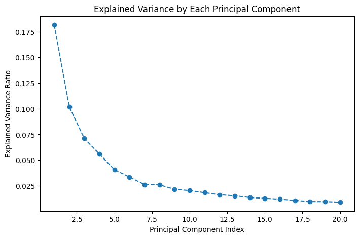
Explained variance ratio of components:  [0.1815466  0.10176539 0.07104166 0.05596602 0.04068942 0.03342151
02613547 0.0258631  0.02152119 0.02033981 0.01828901 0.01626766
01529053 0.01358849 0.01275672 0.01195731 0.01077861 0.00958756
00953736 0.00904233]

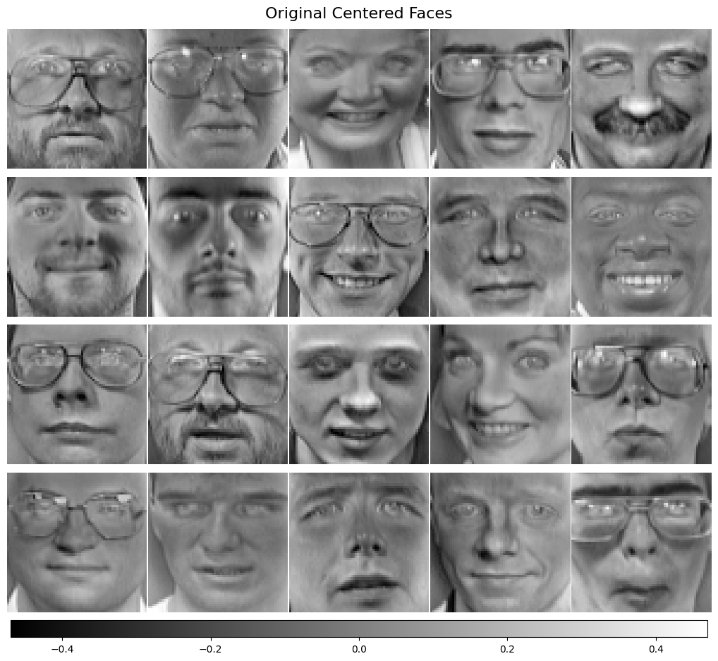
../_images/31c978d0521edd1739fc6fa6e4a2a2bce04ebb8ef1c38600dbcebb4ebc175053.png

In this example, we demonstrate the power of PCA by reconstructing facial images from a low-dimensional representation. The dataset we use is the Olivetti Faces Dataset, which contains images of different individuals’ faces. We start by centering the data both globally (centering each feature, i.e., pixel, across all samples) and locally (centering each sample, i.e., face, across all features). This centering is important for PCA as it ensures that the data has a mean of zero, which simplifies the calculation of principal components.

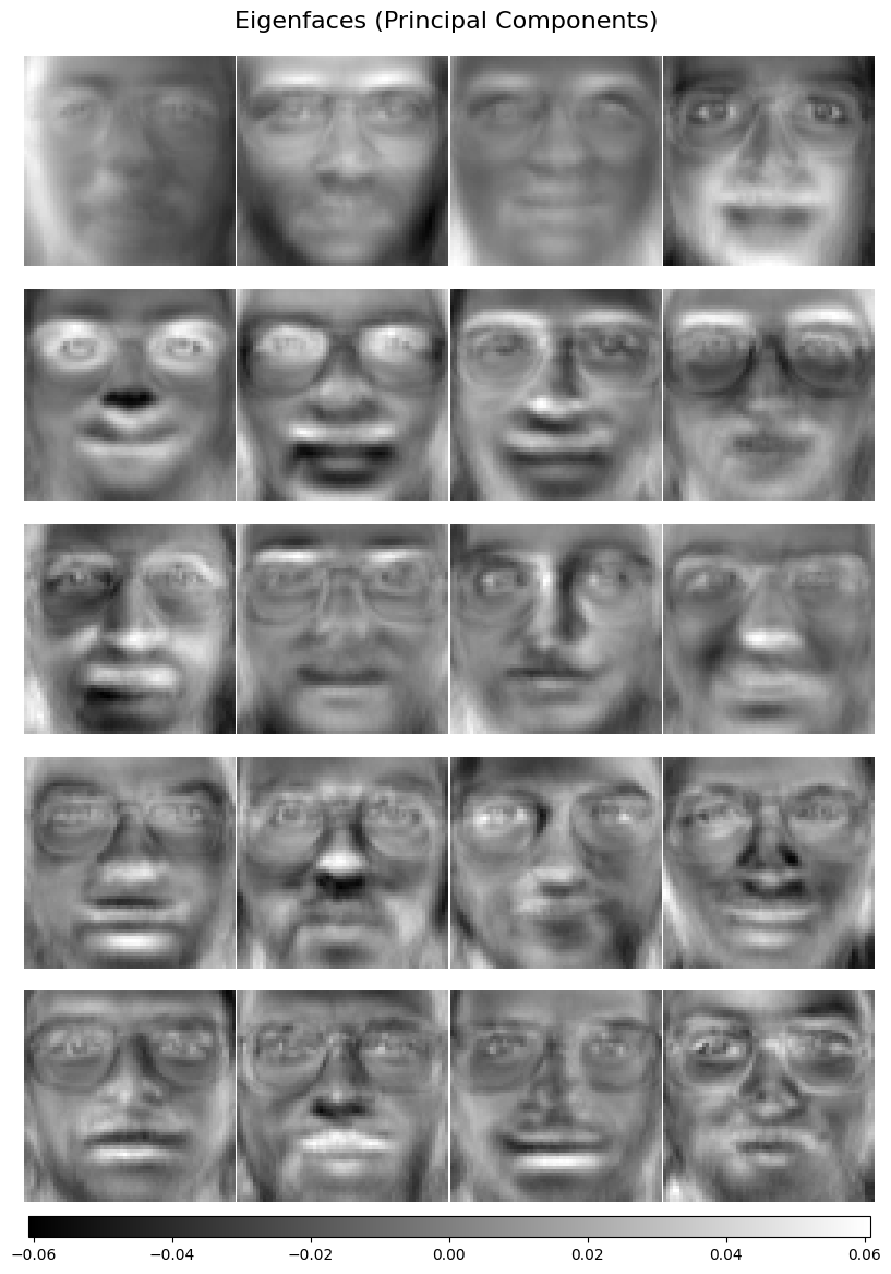
We fit a PCA model to this dataset to extract the eigenfaces, which are the principal components of the dataset. These eigenfaces represent the directions of maximum variance in the face dataset. Each eigenface can be thought of as a building block that captures a certain pattern or feature common across the set of faces (e.g., eyes, nose, or general facial structure).

Interestingly, each of these principal components (eigenfaces) can be interpreted much like the gene-specific effects mentioned previously. In this analogy, the pixel values across all images act as the pixel-specific effects, describing how much each pixel contributes to the overall variation seen across all faces. These effects are then paired with the photo-specific (or sample-specific) coefficients that indicate how much each individual’s face is influenced by these pixel-specific patterns. This combination allows for both general facial patterns and individual differences to be represented efficiently.

Next, we project the original face images onto the lower-dimensional space defined by these eigenfaces. This projection reduces the dimensionality of each face, essentially transforming each high-resolution face image into a vector of only 20 numbers (as we used 20 components in the example). This significant reduction highlights how much the essential features of the faces can be compactly represented.

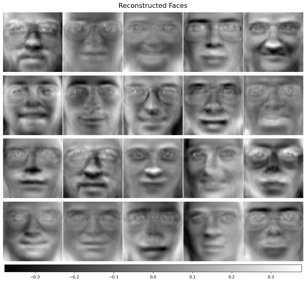
After projecting the faces into the lower-dimensional space, we reconstruct the faces by reversing the process (using the inverse transform). The reconstructed faces are approximate versions of the original ones, created by the linear combination of the eigenfaces weighted by the projection coefficients.

Although the reconstructed faces might not be perfect replicas of the originals, it is important to note that they are generated from only 20 floating-point values, rather than the full set of 4,096 pixel values. This shows the power of PCA in compressing information while retaining the essential features. The reconstructed faces still maintain recognizable traits, despite the massive reduction in data.

We also plotted the explained variance ratio for each of the principal components. This plot helps us understand how much of the total variance in the data is captured by each component. The first few components capture the most significant variation, while the remaining components capture progressively less. This cumulative understanding of variance helps in deciding how many components are necessary for a reasonable reconstruction.

Overall, this example of eigenfaces shows how PCA can reduce the dimensionality of complex data like facial images while retaining meaningful patterns. It highlights PCA’s utility in tasks like compression, noise reduction, and feature extraction, which are common in various machine learning and other data science applications.

	Sample \(1\)	Sample \(2\)	Sample \(3\)		Sample \(M\)	Gene specific \(\mathbf{u}^{(1)}\)	Gene specific \(\mathbf{u}^{(2)}\)
Gene \(1\)	\(X_{11}\)	\(X_{12}\)	\(X_{13}\)	\(\ldots\)	\(X_{1M}\)	\(u^{(1)}_1\)	\(u^{(2)}_1\)
Gene \(2\)	\(X_{21}\)	\(X_{22}\)	\(X_{23}\)	\(\ldots\)	\(X_{2M}\)	\(u^{(1)}_2\)	\(u^{(2)}_2\)
Gene \(3\)	\(X_{31}\)	\(X_{32}\)	\(X_{33}\)	\(\ldots\)	\(X_{3M}\)	\(u^{(1)}_3\)	\(u^{(2)}_3\)
\(\vdots\)	\(\vdots\)	\(\vdots\)	\(\vdots\)	\(\ddots\)	\(\vdots\)	\(\vdots\)	\(\vdots\)
Gene \(N\)	\(X_{N1}\)	\(X_{N2}\)	\(X_{N3}\)	\(\ldots\)	\(X_{NM}\)	\(u^{(1)}_N\)	\(u^{(2)}_N\)

Sample specific \(\mathbf{v}^{T(1)}\)	\(v^{(1)}_1\)	\(v^{(1)}_2\)	\(v^{(1)}_3\)	\(\ldots\)	\(v^{(1)}_M\)	\(S_1\)
Sample specific \(\mathbf{v}^{T(2)}\)	\(v^{(2)}_1\)	\(v^{(2)}_2\)	\(v^{(2)}_3\)	\(\ldots\)	\(v^{(2)}_M\)		\(S_2\)