3. Regularization#
3.1. Introduction to Regularization#
While linear regression works well in many cases, it can suffer from overfitting when the model becomes too complex or the dataset contains noise. Overfitting occurs when a model captures not only the true underlying pattern but also random fluctuations or noise in the data. This leads to poor generalization on unseen data.
One way to combat overfitting is to apply regularization, which modifies the loss function by adding a penalty for large model parameters. The idea is to constrain the model’s flexibility and encourage simpler models that generalize better.
In this chapter, we will introduce two commonly used regularization techniques:
Ridge Regression (also known as L2 regularization)
LASSO Regression (also known as L1 regularization)
3.2. Ridge Regression (L2 Regularization)#
In ridge regression, we modify the ordinary least squares loss function by adding a penalty proportional to the square of the parameters’ magnitudes. This penalty discourages large parameters, leading to a smoother model that is less likely to overfit.
The objective function for ridge regression is:
Where:
\(\lambda\) is a regularization parameter that controls the strength of the penalty. When \(\lambda = 0\), ridge regression reduces to ordinary least squares. As \(\lambda\) increases, the penalty becomes stronger.
\(\beta_j\) are the model parameters (excluding the intercept).
The key idea here is that by penalizing the size of the parameters, we shrink them toward zero, which can help mitigate overfitting.
3.2.1. Ridge Regression Using Scikit-learn#
The scikit-learn package provides a Ridge class that implements ridge regression. Below is an example of how to apply ridge regression to a dataset.
from scipy.optimize import minimize
import numpy as np
import seaborn as sns
import matplotlib.pyplot as plt

# Generate synthetic data
rng = np.random.RandomState(1)
N=20
x = rng.rand(N)
y_non_linear = np.sin(10.*x) + 0.1 * rng.randn(N)
y_non_linear = 4 * x**2 - 10 * x**4  + 6 * x**6 + 0.1 * rng.randn(N)

# Define the polynomial model function
def polynomial_model(x, params, degree=7):
    x_poly = np.vstack([x**i for i in range(degree + 1)]).T
    return np.dot(x_poly, params)

def minimize_loss(loss, model, x, y, num_params):
    initial_params = np.random.randn(num_params)
    return minimize(loss, initial_params, args=(model, x, y))

def rss_loss(params, model_function, X, y):
    predictions = model_function(x, params)  # Predicted values
    residual_sum_squares = np.sum((y - predictions) ** 2)  # RSS
    return residual_sum_squares

# Define ridge loss function
def ridge_loss(params, model_function, X, y, alpha=0.1):
    residual_sum_squares =  rss_loss(params, model_function, X, y)  # RSS
    l2_penalty = alpha * np.sum(params**2)
    return residual_sum_squares + l2_penalty

# Optimize the parameters of our model using the ridge loss function
result_poly_rss = minimize_loss(rss_loss, polynomial_model, x, y_non_linear,8)
result_poly_ridge = minimize_loss(ridge_loss, polynomial_model, x, y_non_linear,8)

poly_params_rss = result_poly_rss.x
poly_params_ridge = result_poly_ridge.x

# Generate fit lines
xfit = np.linspace(np.min(x), np.max(x), 1000)
yfit_poly_rss = polynomial_model(xfit, poly_params_rss)
yfit_poly_ridge = polynomial_model(xfit, poly_params_ridge)

sns.scatterplot(x=x, y=y_non_linear, label="Data")
plt.plot(xfit, yfit_poly_rss, color='r',label="RSS")
plt.plot(xfit, yfit_poly_ridge, color='b',label="Ridge")
plt.legend()
plt.show()

print("Polynomial parameters (RSS):", poly_params_rss)
print("Polynomial parameters (Ridge):", poly_params_ridge)
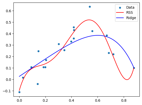
Polynomial parameters (RSS): [-9.71256700e-02  3.97695982e+00 -2.88397239e+01  9.51218084e+01
 -1.06709009e+02 -7.68457731e+00  6.23537909e+01 -1.63772256e+01]
Polynomial parameters (Ridge): [ 0.0257251   0.75907553  0.0711282  -0.21788742 -0.29144466 -0.27566192
 -0.23087908 -0.18251898]
In this example, alpha corresponds to \(\lambda\) and controls the regularization strength. By tuning this parameter, we can adjust the model’s complexity.
3.3. LASSO Regression (L1 Regularization)#
LASSO regression (Least Absolute Shrinkage and Selection Operator) is another regularization technique. Instead of penalizing the sum of squared parameters, LASSO penalizes the sum of the absolute values of the parameters. This results in sparse solutions, where some of the parameters may become exactly zero.
The objective function for LASSO regression is:
Where:
\(\lambda\) again controls the regularization strength.
The absolute value penalty leads to sparse models, meaning that LASSO can perform feature selection by setting some parameters to zero.
LASSO is particularly useful when we have many features, as it can identify and retain only the most important ones.
3.3.1. LASSO Regression Using Scikit-learn#
The scikit-learn package provides a Lasso class for L1-regularized regression. Below is an example of LASSO applied to a dataset.
import numpy as np
import matplotlib.pyplot as plt
import seaborn as sns
from scipy.optimize import minimize

# Define LASSO loss function
def lasso_loss(params, model_function, X, y, alpha=0.1):
    residual_sum_squares =  rss_loss(params, model_function, X, y)  # RSS
    l1_penalty = alpha * np.sum(np.abs(params))  # L1 regularization
    return residual_sum_squares + l1_penalty

# Optimize the parameters of our model using the lasso loss function
result_poly_lasso = minimize_loss(lasso_loss, polynomial_model, x, y_non_linear,8)

poly_params_lasso = result_poly_lasso.x

# Generate fit lines
yfit_poly_lasso = polynomial_model(xfit, poly_params_lasso)

sns.scatterplot(x=x, y=y_non_linear, label="Data")
plt.plot(xfit, yfit_poly_rss, color='r',label="RSS")
plt.plot(xfit, yfit_poly_lasso, color='b',label="LASSO")
plt.legend()
plt.show()

# Print parameters
print("Polynomial parameters (RSS):", poly_params_rss)
print("Polynomial parameters (LASSO):", poly_params_lasso)
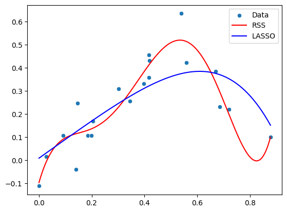
Polynomial parameters (RSS): [-9.71256700e-02  3.97695982e+00 -2.88397239e+01  9.51218084e+01
 -1.06709009e+02 -7.68457731e+00  6.23537909e+01 -1.63772256e+01]
Polynomial parameters (LASSO): [ 8.92554013e-03  8.13386916e-01 -7.07532084e-09 -1.92909997e-01
 -1.31629483e-01 -6.86516342e-01 -9.57827073e-03 -2.24275647e-08]
As with ridge regression, alpha controls the strength of regularization. When \(\alpha\) is large, more parameters will be set to values close to zero, resulting in a simpler model. It is worth noting that there are better optimization schemes available than regular gradient decent optimizers specially targeting LASSO regression, which helps keeping parameters at exactly 0 (not just close to 0).
3.4. Comparing Ridge and LASSO#
While both ridge and LASSO regression aim to reduce overfitting by penalizing large parameters, they behave differently:
Ridge regression tends to shrink parameters but rarely sets them exactly to zero. This means that it keeps all features in the model, but the influence of less important features is reduced.
LASSO regression, on the other hand, can shrink parameters all the way to zero, effectively performing feature selection.
The choice between ridge and LASSO depends on the problem:
If you believe that all features are relevant and you want to shrink their influence, ridge might be the better option.
If you suspect that only a few features are truly important, LASSO can help by selecting those features automatically.
3.5. Elastic Net: Combining Ridge and LASSO#
In some cases, it can be beneficial to combine the strengths of ridge and LASSO regression. This is achieved with Elastic Net, which includes both L1 and L2 penalties.
The objective function for Elastic Net is:
Here, both \(\lambda_1\) and \(\lambda_2\) control the balance between L1 and L2 regularization. This method is particularly useful when there are correlations between features, as it can encourage a grouping effect, where correlated features tend to have similar parameters.
3.5.1. Elastic Net Using Scikit-learn#
The scikit-learn package also provides an ElasticNet class, which combines ridge and LASSO regularization.
from sklearn.linear_model import ElasticNet

# Fit Elastic Net model
x_poly = np.vstack([x**i for i in range(8)]).T
elastic_net_model = ElasticNet(alpha=0.005, l1_ratio=0.5)  # l1_ratio controls the balance between L1 and L2 regularization
elastic_net_model.fit(x_poly, y_non_linear)

# Predict and plot
x_poly_fit = np.vstack([xfit**i for i in range(8)]).T
yfit_elastic_net = elastic_net_model.predict(x_poly_fit)

sns.scatterplot(x=x, y=y_non_linear, label="data")
plt.plot(xfit, yfit_elastic_net, color='m', label="elastic net")
plt.legend()
plt.show()
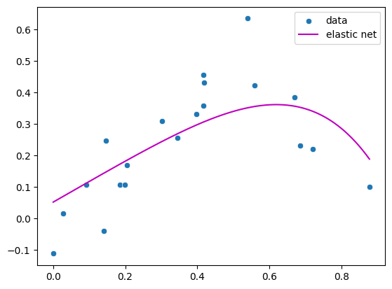
By tuning both the alpha and l1_ratio parameters, we can control the balance between ridge and LASSO regularization.
3.6. Why Does This Work?#
Regularization works by reducing the likelihood of overfitting through the addition of penalties for large model parameters. In regression models, parameters represent the strength and direction of the relationship between each feature and the target variable. When these parameters grow large, it can indicate that the model is reacting too strongly to specific details or noise in the training data, which may not hold for new data. This is a sign of overfitting: the model has not only learned the true underlying patterns but has also fit itself to random fluctuations or specific data instances in the training set.
By adding penalties (as in L1 and L2 regularization), we shrink the size of the parameters. Smaller parameters prevent the model from placing too much importance on any one feature unless it truly adds significant predictive value. In L2 regularization (Ridge), for example, parameters are constrained by a penalty on their squared magnitudes, which promotes a smoother fit and reduces the model’s flexibility. L1 regularization (Lasso), on the other hand, may drive some parameters all the way to zero, effectively performing feature selection and allowing the model to focus only on the most important predictors.
This constraint on parameter size simplifies the model, reducing its tendency to memorize the training data and helping it generalize better to unseen data. By focusing on essential relationships, regularization leads the model to capture the overall trend or signal in the data, rather than noise, enhancing its robustness and predictive power across different datasets.
Here is a short section you can insert into your book text on why we refer to L1 and L2 regularization.
3.6.1. Why “L1” and “L2” Regularization?#
The labels “L1” and “L2” come from the notation of vector norms in mathematics. A norm on a vector space is a function that assigns a non-negative length or size to each vector and satisfies certain axioms (positivity, homogeneity, triangle inequality). The L1 norm (also written \(\ell_1\)-norm) of a vector \(w = (w_1, w_2, \dots, w_p)\) is
The L2 norm (or (\ell_2)-norm) is
which corresponds geometrically to the Euclidean length of the vector.