11. Hypothesis Testing#
Hypothesis testing is a statistical procedure used to determine if a sample data set provides sufficient evidence to reject a stated null hypothesis (\(H_0\)) in favor of an alternative hypothesis (\(H_1\)). This method is fundamental in science for drawing inferences about populations based on sample data. It allows researchers to make data-driven decisions and evaluate the likelihood that their observations are due to random chance or a genuine effect.
11.1. Statistical hypothesis test#
11.1.1. Null Hypothesis (\(H_0\)) and Alternative Hypothesis (\(H_1\))#
In hypothesis testing, we begin by stating two competing hypotheses about population or a set of populations:
Null Hypothesis (\(H_0\)): This is a statement suggesting there is no effect, relationship, or difference. It represents the status quo or a baseline assumption. For example, in a clinical trial, \(H_0\) might state that a new drug has no effect compared to a placebo (i.e. the patients in placebo population are not different than the one in the population of treated patients).
Alternative Hypothesis (\(H_1\)): This hypothesis reflects what the researcher aims to prove. It suggests that there is an effect, a relationship, or a difference. In the clinical trial example, \(H_1\) would state that the new drug has a beneficial effect compared to the placebo.
The purpose of hypothesis testing is to assess whether the data provides enough evidence to reject \(H_0\) in favor of \(H_1\). This process involves comparing the observed data in a sample to what we would expect under \(H_0\).
11.1.2. Test Statistics#
A test statistic is a value calculated from sample data that allows us to make a decision about the hypotheses. One commonly used test statistic is the difference in means between two samples. For example, if we want to compare the average effect of a treatment versus a placebo, we calculate the difference in the sample means for the two groups. The test statistic helps determine how far the observed data deviates from what we would expect under \(H_0\), which typically assumes that there is no difference in means between the groups.
11.1.3. Sampling Distribution under the Null Hypothesis#
The sampling distribution under the null hypothesis is the distribution of the test statistic assuming that \(H_0\) is true. This distribution helps us understand the range of possible values the test statistic can take if the null hypothesis is correct. By comparing the observed test statistic to this distribution, we can determine how likely it is to observe such a value by random chance alone. This comparison is essential for calculating the p value.
11.2. \(p\) value#
The \(p\) value represents the probability of obtaining the observed data, or something more extreme, if the null hypothesis were true. It is used as a measure of evidence against \(H_0\):
A smaller \(p\) value suggests that the observed data would be unlikely under \(H_0\), providing stronger evidence against the null hypothesis.
For example, a \(p\) value of 0.03 means there is a 3% chance of observing the data (or something more extreme) if \(H_0\) is true. This small probability indicates that the data is not consistent with \(H_0\), leading us to consider rejecting it.
11.2.1. Significance Level (\(\alpha\))#
The significance level (denoted as \(\alpha\)) is a predetermined threshold that determines whether the p value is considered small enough to reject the null hypothesis. A common choice for \(\alpha\) is 0.05, which means we are willing to accept a 5% chance of incorrectly rejecting \(H_0\) (Type I error):
If the p value is less than \(\alpha\), the results are considered statistically significant, and we reject \(H_0\).
The choice of \(\alpha\) depends on the context of the study and the consequences of making an error. For example, in medical research, a smaller \(\alpha\) (e.g., 0.01) might be chosen to reduce the risk of false positives.
11.2.2. False Positives and False Negatives#
In hypothesis testing, two types of errors can occur:
False Positive (Type I Error): Rejecting \(H_0\) when it is actually true. This error can lead to incorrect conclusions, such as believing a treatment is effective when it is not.
False Negative (Type II Error): Failing to reject \(H_0\) when the alternative hypothesis is true. This error can result in missed discoveries, such as failing to detect a real effect or relationship.
The balance between Type I and Type II errors is crucial in hypothesis testing. Researchers often need to consider the trade-offs between these errors when designing studies and choosing significance levels.
11.2.3. Limitations & Misinterpretations#
While hypothesis testing is powerful, it has its limitations and can be easily misinterpreted:
\(p\) values provide the strength of evidence against \(H_0\), but they do not indicate the size of the effect or its practical significance. A small \(p\) value might suggest a statistically significant result, but the actual effect size could be trivial.
A \(p\) value does not give the probability that either hypothesis is true. It only tells us how compatible the observed data is with \(H_0\).
Results can be statistically significant without being practically significant, and vice versa. Thus, it is crucial to interpret the results in the context of the research question and the real-world implications. For instance, a medical treatment might show a statistically significant improvement, but the actual benefit to patients might be minimal.
11.3. Assessing Significance Using Permutation Testing#
We can use permutation testing to evaluate significance. This approach involves creating a null distribution by permuting the dependent variable (the target) and calculating the corresponding loss values. We then compare the observed loss to this distribution to compute a \(p\) value.
11.3.1. Why Permutation Testing?#
Permutation testing is non-parametric, meaning it doesn’t assume a specific distribution of the residuals or the coefficients. This makes it a powerful and flexible method, especially in cases where the assumptions of parametric tests (e.g., normality) might not hold. Further, we here use it as a pedagogic tool, to understand how frequentist hypothesis testing actually works.
11.4. Permutation Testing for Model Significance#
In permutation testing, we test the null hypothesis that there is no relationship between the dependent and independent variables. To do this, we randomly shuffle the dependent variable \(y\) while keeping the independent variable \(\mathbf{x}\) unchanged, refit the model, and compute the loss. Repeating this process many times creates a null distribution of losses. The \(p\) value is calculated by comparing the observed loss to this null distribution. The idea is that if we are testing the association between \(\mathbf{x}\) and \(y\), then under the null hypothesis, any random pairing between \(\mathbf{x}\) and \(y\) should have the same effect on the model as the actual observed pairing.
11.4.1. Step-by-step Procedure#
Fit the model on the original data and calculate the observed loss.
Permute the dependent variable (shuffle y) and refit the model on the permuted data to calculate the loss under the null hypothesis.
Repeat the permutation process many times to build a distribution of losses under the null hypothesis.
Calculate the \(p\) value by comparing the observed loss to this distribution.
11.4.2. Code Example: Permutation Test for comparing means of two populations#
Below is an example of how to implement permutation testing for assessing the significance of differences between two samples.
import numpy as np
import seaborn as sns
import matplotlib.pyplot as plt
# Generate two normally distributed samples with slightly different means
rng = np.random.RandomState(2)
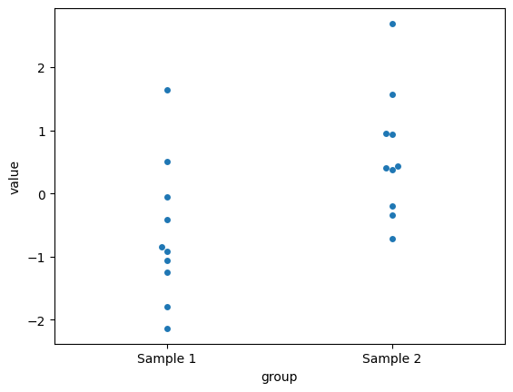
sample1 = rng.normal(loc=0.0, scale=1.0, size=10)
sample2 = rng.normal(loc=0.4, scale=1.0, size=10)
# Plot the samples using swarmplot
data = {'value': np.concatenate([sample1, sample2]),
'group': ['Sample 1'] * len(sample1) + ['Sample 2'] * len(sample2)}
sns.swarmplot(x='group', y='value', data=data)
plt.show()
# Permutation test for difference in means
n_permutations = 1000
observed_diff = np.abs(np.mean(sample1) - np.mean(sample2))
combined = np.concatenate([sample1, sample2])
permuted_diffs = []
for _ in range(n_permutations):
permuted = rng.permutation(combined)
perm_sample1 = permuted[:len(sample1)]
perm_sample2 = permuted[len(sample1):]
permuted_diff = np.abs(np.mean(perm_sample1) - np.mean(perm_sample2))
permuted_diffs.append(permuted_diff)
# Compute the p-value by comparing the observed difference to the null distribution
permuted_diffs = np.array(permuted_diffs)
p_value = np.mean(permuted_diffs >= observed_diff)
# Plot the null distribution and observed difference
plt.hist(permuted_diffs, bins=30, alpha=0.7, label="Permuted Differences")
plt.axvline(observed_diff, color='r', linestyle='--', label=f"Observed Diff = {observed_diff:.2f}")
plt.title(f"Permutation Test for Difference in Means (p-value = {p_value:.4f})")
plt.xlabel("Difference in Means")
plt.ylabel("Frequency")
plt.legend()
plt.show()
print(f"Observed difference in means: {observed_diff:.4f}")
print(f"p-value from permutation test: {p_value:.4f}")
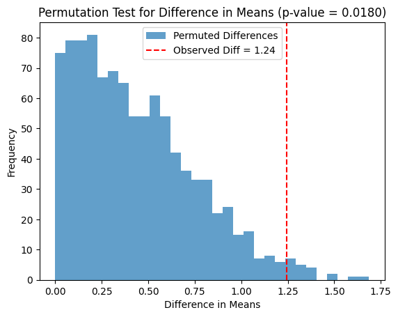
Observed difference in means: 1.2441
p-value from permutation test: 0.0180
11.4.3. Permutation Test for Model Significance#
Below is an example of how to implement permutation testing for assessing the significance of a regression model. Here we use the SSE of the model as a test statistics.
import numpy as np
from scipy.optimize import minimize
import seaborn as sns
import matplotlib.pyplot as plt

# Generate synthetic data
rng = np.random.RandomState(42)
x = rng.rand(50)
y = 1.2 * x - 0.5 + 1.1 * rng.randn(50)

# Define the linear model
def linear_model(params, x):
    slope, intercept = params
    return slope * x + intercept

# Define the loss function (sum of squared residuals)
def loss(params, x, y):
    return np.sum((y - linear_model(params, x))**2)

# Fit the model to the original data
initial_params = np.random.randn(2)
result = minimize(loss, initial_params, args=(x, y))
observed_loss = result.fun

# Permutation test
n_permutations = 1000
permuted_losses = []

for _ in range(n_permutations):
    # Shuffle y and fit the model to the permuted data
    y_permuted = np.random.permutation(y)
    permuted_result = minimize(loss, initial_params, args=(x, y_permuted))
    permuted_losses.append(permuted_result.fun)

# Compute the p-value by comparing the observed loss to the null distribution
permuted_losses = np.array(permuted_losses)
p_value = np.mean(permuted_losses <= observed_loss)

# Plot the null distribution and observed loss
plt.hist(permuted_losses, bins=30, alpha=0.7, label="Permuted Losses")
plt.axvline(observed_loss, color='r', linestyle='--', label=f"Observed Loss = {observed_loss:.2f}")
plt.title(f"Permutation Test for Model Significance (p-value = {p_value:.4f})")
plt.xlabel("SSE Loss")
plt.ylabel("Frequency")
plt.legend()
plt.show()

print(f"Observed loss: {observed_loss:.4f}")
print(f"p value from permutation test: {p_value:.4f}")
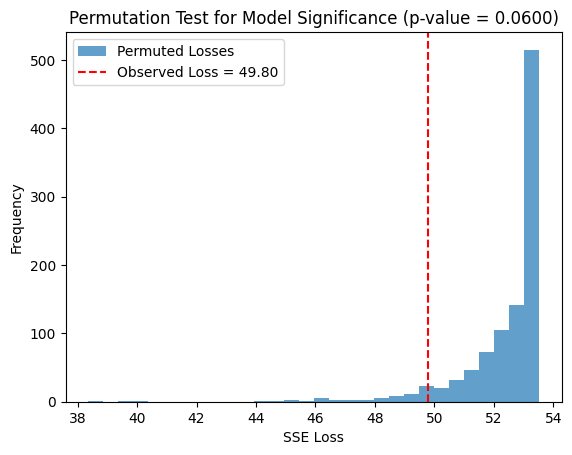
Observed loss: 49.7958
p value from permutation test: 0.0600
11.5. t-tests#
When the population from which your samples are drawn is normally distributed, a t-test can be used to evaluate whether there is a significant difference between the means of two independent groups. Under these conditions, the sampling distribution of the difference in means follows a t-distribution, which allows us to calculate the probability (p-value) of observing a difference as large as (or larger than) the one obtained, assuming the null hypothesis is true.
Below is a Python script demonstrating how to perform a t-test on two sample datasets using the SciPy library.
import numpy as np
from scipy.stats import ttest_ind

# Generate synthetic data for two independent samples

# Perform a two-sample t-test (on the same sample we used previously)
t_stat, p_value = ttest_ind(sample1, sample2)

print(f"P-value: {p_value:.4f}")
P-value: 0.0168
When we assume normality, as in t-tests, we gain sensitivity, especially for smaller sample sizes. The t-test uses the properties of the t-distribution to calculate p-values, and this assumption provides more power to detect differences when data truly follow a normal distribution. For smaller sample sizes, this assumption becomes particularly advantageous because the t-test can yield lower p-values, allowing subtle differences to be detected more effectively. However, if the assumption of normality is violated, the accuracy of the p-values is compromised, which could lead to misleading conclusions. This sensitivity-robustness trade-off is especially important in small-sample scenarios.
11.6. One- vs Two-sided tests#
Here’s a brief explanation of the difference between one-sided and two-sided tests:
A one-sided test is used when we want to determine if there is a difference in a specific direction (e.g., whether one group mean is greater than the other). In contrast, a two-sided test checks if there is any difference between the groups, regardless of direction (i.e., whether one mean is greater or less than the other). A two-sided test is more conservative because it tests for deviations in both directions, while a one-sided test focuses on a predetermined outcome.
Here’s how you could modify the permutation test to be one-sided for comparing sample1 and sample2, checking if sample2 has a larger mean:
import numpy as np
import seaborn as sns
import matplotlib.pyplot as plt
from IPython.display import display, Markdown, Math

# Generate two normally distributed samples with slightly different means
rng = np.random.RandomState(42)
sample1 = rng.normal(loc=0.0, scale=1.0, size=10)
sample2 = rng.normal(loc=0.5, scale=1.0, size=10)

# Plot the samples using swarmplot
data = {'value': np.concatenate([sample1, sample2]),
        'group': ['Sample 1'] * len(sample1) + ['Sample 2'] * len(sample2)}

sns.swarmplot(x='group', y='value', data=data)
plt.title('Swarmplot of Two Samples')
plt.show()

# One-sided permutation test for difference in means (Sample 2 > Sample 1)
n_permutations = 1000
observed_diff = np.mean(sample2) - np.mean(sample1)

combined = np.concatenate([sample1, sample2])
permuted_diffs = []

for _ in range(n_permutations):
    permuted = rng.permutation(combined)
    perm_sample1 = permuted[:len(sample1)]
    perm_sample2 = permuted[len(sample1):]
    permuted_diff = np.mean(perm_sample2) - np.mean(perm_sample1)
    permuted_diffs.append(permuted_diff)

# Compute the p-value by comparing the observed difference to the null distribution (one-sided)
permuted_diffs = np.array(permuted_diffs)
ge_p_value = np.mean(permuted_diffs >= observed_diff)
le_p_value = np.mean(permuted_diffs <= observed_diff)
two_p_value = np.mean(abs(permuted_diffs) >= abs(observed_diff))

# Plot the null distribution and observed difference
plt.hist(permuted_diffs, bins=30, alpha=0.7, label="Permuted Differences")
plt.axvline(observed_diff, color='r', linestyle='--', label=f"Observed Diff = {observed_diff:.2f}")
plt.xlabel("Difference in Means")
plt.ylabel("Frequency")
plt.legend()
plt.show()

display(Markdown(rf"Observed difference in means: {observed_diff:.4f}"))
display(Math(rf"p (H_0: \Delta \le 0): {ge_p_value:.4f}"))
display(Math(rf"p (H_0: \Delta \ge 0): {le_p_value:.4f}"))
display(Math(rf"p (H_0: \Delta = 0): {two_p_value:.4f}"))
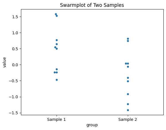
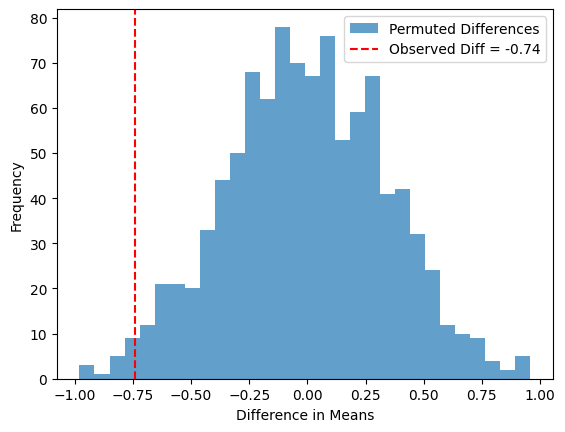
Observed difference in means: -0.7387
In this one-sided permutation test, we are specifically testing if sample2 has a larger mean than sample1. The observed difference and permuted differences are not taken as absolute values, and the p-value is computed based on the proportion of permutations where perm_sample2 - perm_sample1 is greater than or equal to the observed difference. This makes it a one-sided test focusing on whether sample2 is greater (or smaller) than sample1.
If you test the efficiency of a drug, you are usually interested in whether the drug has a positive effect on patients, without considering whether it could have a negative effect. In such cases, a one-sided test is appropriate. On the other hand, in differential gene expression analysis, you often want to investigate both upregulation and downregulation of genes between patient groups, making a two-sided test more suitable.
11.7. Overview of the workflow in frequentist testing procedures#
        graph TD
    A(Population, μ ) --> B[Sample, X̄]
    B --> C[Statistical Model, μ - X̄]
    C -.->|Inference about
    population parameter μ | A
The diagram represents the process of statistical inference from a population to a sample and back. The key steps are:
Population: The population contains all the members of interest, and we are interested in a particular population parameter, here represented by μ. This could be a measure like the mean or proportion that describes the entire population.
Sample: We draw a sample from the population, and from this sample, we calculate a statistic, here denoted as X̄. The statistic serves as an estimate of the population parameter. However, this estimate may include sampling errors, which result from the fact that the sample is only a subset of the full population, as well as measurement errors.
Statistical Model: A statistical model is built to describe the relationship between the statistic (X̄) and the population parameter (μ). This model helps us quantify uncertainty, and potentially correct for errors or biases, and ultimately use sample information to make inferences about the population.
Inference about Population Parameter: Using the statistical model, we then make inferences about the population parameter. The goal is to make a statements about the true value of the population parameter (μ), based on the information contained in the sample and the statistical modeling of the errors.
11.8. Volcano Plots and Their Interpretation#
A volcano plot is a type of scatter plot commonly used in genomics, proteomics, and other fields of biology to display the results of differential expression or differential abundance analysis. The plot provides a clear visual summary of large datasets, making it easier to identify statistically significant changes between two experimental conditions.
On a volcano plot:
The x-axis represents the fold change (often as a log2 value) between two groups, showing the magnitude of change in expression or abundance.
The y-axis represents the statistical significance (usually as the negative log10 of the p-value) of that change.
Points that are:
Farther to the left or right indicate larger fold changes.
Higher on the y-axis indicate more significant p-values.
Data points that fall at the extremes of both axes are of most interest, as they represent features (e.g., genes or proteins) that have both a large effect size (strong change) and high statistical confidence.
The name “volcano plot” arises from the characteristic shape, where the data points resemble an erupting volcano. Features with statistically significant, biologically meaningful changes are generally those that lie far from the center, either on the left or right.
11.8.1. Example Script for Generating a Volcano Plot#
Here’s a Python script that generates random data to create a volcano plot:
import pandas as pd
import matplotlib.pyplot as plt
from scipy.stats import ttest_ind

# Parameters
num_genes = 1000
sample_size = 5
mu, sigma = 4.0, 0.5

# Random number generator
rng = np.random.RandomState(42)

# Generate data for each gene
gene_data = []
for i in range(num_genes):
    # Sample an offset for each gene from a normal distribution
    offset = rng.normal(0., 1.)

    # Generate two samples with the offset
    sample1 = rng.normal(mu, sigma, sample_size)
    sample2 = rng.normal(mu + offset, sigma, sample_size)

    # Calculate fold change as the difference in means (log2)
    fold_change = np.log2(np.mean(sample2)) - np.log2(np.mean(sample1))

    # Perform a t-test to calculate p-value
    _, p_value = ttest_ind(sample1, sample2, alternative='two-sided')

    # Store the gene data
    gene_data.append([fold_change, p_value])

# Create DataFrame
data = pd.DataFrame(gene_data, columns=['FoldChange', 'PValue'])

# Convert p-values to -log10(p-value)
data['negLog10PValue'] = -np.log10(data['PValue'])

# Create the volcano plot
plt.figure(figsize=(10, 6))
plt.scatter(data['FoldChange'], data['negLog10PValue'], alpha=0.6, edgecolors='w', linewidth=0.5)
plt.axhline(-np.log10(0.05), color='red', linestyle='--', label='p-value = 0.05')
plt.axvline(-1, color='blue', linestyle='--', label='Fold Change = -1')
plt.axvline(1, color='blue', linestyle='--', label='Fold Change = 1')

plt.xlabel('Log2 Fold Change')
plt.ylabel('-Log10 p-value')
plt.title('Volcano Plot of Simulated Gene Data')
plt.legend()
plt.show()
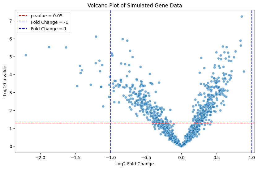
This script simulates random fold changes and p-values to illustrate a volcano plot:
The x-axis shows log2-transformed fold changes.
The y-axis shows the negative log10-transformed p-values.
The red horizontal line indicates a significance threshold (p-value = 0.05).
The blue vertical lines represent log2 fold changes of ±1, which could be used as an effect size threshold.
This example shows how points that meet both criteria (large fold change and significant p-value) can be visually highlighted, making volcano plots a useful tool for identifying important differences in biological studies. Note that we have not corrected for multiple testing when performing these tests, something we will discuss in a separate chapter (and lecture).