Multi-Layer Perceptrons (MLPs)

10. Multi-Layer Perceptrons (MLPs)#

A Multi-Layer Perceptron (MLP) is a class of feedforward artificial neural network. An MLP consists of at least three layers: an input layer, one or more hidden layers, and an output layer. Each layer is fully connected to the next, and the network is trained using backpropagation to adjust the weights based on the error.

MLPs are widely used in supervised learning tasks such as classification and regression. They can model complex, non-linear relationships between input and output by stacking multiple layers of neurons.

10.1. Artificial Neuron#

An artificial neuron is a fundamental building block of neural networks. It is inspired by the biological neuron and functions as a mathematical model that takes multiple inputs, processes them, and produces an output. The artificial neuron makes a linear combination of its input that is forwarded to a non-linear activation function. This can be expressed as:

\[ f(\mathbf{x};\mathbf{w}) = g(\sum_{i=1}^n w_i x_i + b) \]

This expression can be broken down into these two steps:

Linear combination: Each input is multiplied by a weight, and then all the weighted inputs are summed together. Additionally, a bias term is added to the sum. Mathematically, this can be represented as:

\[ z = \sum_{i=1}^n w_i x_i + b \]

Where:

\(x_i\) are the inputs
\(w_i\) are the weights
\(b\) is the bias term

Activation Function: The weighted sum is passed through an activation function, \(g(x)\), to introduce non-linearity. Common activation functions include:
- Sigmoid: Maps the input to a value between 0 and 1.
- ReLU (Rectified Linear Unit): Sets all negative values to zero and passes positive values unchanged.
- Tanh: Maps the input to a value between -1 and 1.

10.2. Components of an MLP#

The output of the activation function becomes the output of the neuron, which can then be used as input to other neurons.

../_images/mlp.svg — Fig. 10.1 An example MLP. Each layer of the MLP consists of a set of artificial neurons, that receive input from the previous layer, process it, and pass the output to the next layer.#

Input Layer: The input layer consists of neurons that receive the raw data. Each neuron in the input layer represents a feature of the input data.
Hidden Layers: Between the input and output layers are one or more hidden layers. Neurons in the hidden layers receive input from the previous layer, process it, and pass the output to the next layer. Adding more hidden layers allows the network to learn more complex relationships in the data.
Output Layer: The output layer produces the final prediction or classification. The number of neurons in this layer depends on the type of task (e.g., a single neuron for binary classification or multiple neurons for multi-class classification).

Neurons in each layer are fully connected to neurons in the subsequent layer, meaning each neuron receives input from all neurons in the previous layer. The strength of these connections is determined by the weights, which are adjusted during training to minimize the error between the predicted output and the actual output.

10.3. Training an MLP#

MLPs are trained using backpropagation and gradient descent. The process involves the following steps:

Forward Pass: Input data passes through the network, and predictions are generated.
Loss Calculation: A loss function (e.g., mean squared error for regression or cross-entropy for classification) is used to measure the error between the predictions and true labels.
Backward Pass: Gradients of the loss with respect to the weights are computed, using the chain rule. Weights are the updated using optimization techniques, often gradient descent-based techniques. A more detailed description can be found in the wikipedia entry.

10.4. Example: Training an MLP on Artificial Data#

In this example, we’ll generate artificial data from two non-linearly separable distributions and train an MLP to classify them into two classes.

# Import necessary libraries
import numpy as np
import seaborn as sns
import matplotlib.pyplot as plt
from sklearn.model_selection import train_test_split
from sklearn.datasets import make_moons
from sklearn.metrics import accuracy_score

sns.set_style("whitegrid")

# Generate non-linearly separable data
np.random.seed(0)
X, y = make_moons(n_samples=1000, noise=0.2, random_state=42)

# Split the data into training and test sets
X_train, X_test, y_train, y_test = train_test_split(X, y, test_size=0.3, random_state=42)

# Convert y to a column vector
y_train = y_train.reshape(-1, 1)
y_test = y_test.reshape(-1, 1)

# Define the sigmoid activation function
def sigmoid(z):
    return 1 / (1 + np.exp(-z))

# Derivative of the sigmoid function (needed for backpropagation)
def sigmoid_derivative(z):
    return sigmoid(z) * (1 - sigmoid(z))

# Initialize parameters (weights and biases)
n_hidden_1 = 10
n_hidden_2 = 5
n_input = X_train.shape[1]
n_output = 1

np.random.seed(42)
weights_1 = np.random.randn(n_input, n_hidden_1)  # Input to first hidden layer
bias_1 = np.zeros((1, n_hidden_1))
weights_2 = np.random.randn(n_hidden_1, n_hidden_2)  # First hidden to second hidden layer
bias_2 = np.zeros((1, n_hidden_2))
weights_out = np.random.randn(n_hidden_2, n_output)  # Second hidden to output layer
bias_out = np.zeros((1, n_output))

# Training parameters
learning_rate = 0.01
n_epochs = 1000

# Training loop
for epoch in range(n_epochs):
    # Forward pass: compute activations layer by layer
    z1 = np.dot(X_train, weights_1) + bias_1
    a1 = sigmoid(z1)  # Activation for first hidden layer
    z2 = np.dot(a1, weights_2) + bias_2
    a2 = sigmoid(z2)  # Activation for second hidden layer
    z_out = np.dot(a2, weights_out) + bias_out
    y_pred = sigmoid(z_out)  # Output prediction

    # Compute loss (binary cross-entropy)
    loss = -np.mean(y_train * np.log(y_pred) + (1 - y_train) * np.log(1 - y_pred))

    # Backward pass (gradient computation using chain rule)
    # Gradient of loss w.r.t. output layer activation (y_pred)
    d_loss_y_pred = -(y_train / y_pred) + ((1 - y_train) / (1 - y_pred))
    # Gradient of sigmoid activation w.r.t. z_out (output layer input)
    d_y_pred_z_out = sigmoid_derivative(z_out)
    # Chain rule: Gradient of loss w.r.t. z_out
    d_loss_z_out = d_loss_y_pred * d_y_pred_z_out

    # Gradients for output layer weights and biases
    d_loss_weights_out = np.dot(a2.T, d_loss_z_out)  # Chain rule to propagate to weights
    d_loss_bias_out = np.sum(d_loss_z_out, axis=0, keepdims=True)

    # Propagate the gradient back to the second hidden layer
    d_loss_a2 = np.dot(d_loss_z_out, weights_out.T)  # Gradient w.r.t. activations in second hidden layer
    d_a2_z2 = sigmoid_derivative(z2)
    d_loss_z2 = d_loss_a2 * d_a2_z2  # Gradient w.r.t. z2 (input to second hidden layer)

    # Gradients for second hidden layer weights and biases
    d_loss_weights_2 = np.dot(a1.T, d_loss_z2)
    d_loss_bias_2 = np.sum(d_loss_z2, axis=0, keepdims=True)

    # Propagate the gradient back to the first hidden layer
    d_loss_a1 = np.dot(d_loss_z2, weights_2.T)  # Gradient w.r.t. activations in first hidden layer
    d_a1_z1 = sigmoid_derivative(z1)
    d_loss_z1 = d_loss_a1 * d_a1_z1  # Gradient w.r.t. z1 (input to first hidden layer)

    # Gradients for first hidden layer weights and biases
    d_loss_weights_1 = np.dot(X_train.T, d_loss_z1)
    d_loss_bias_1 = np.sum(d_loss_z1, axis=0, keepdims=True)

    # Update weights and biases using gradients
    weights_out -= learning_rate * d_loss_weights_out
    bias_out -= learning_rate * d_loss_bias_out
    weights_2 -= learning_rate * d_loss_weights_2
    bias_2 -= learning_rate * d_loss_bias_2
    weights_1 -= learning_rate * d_loss_weights_1
    bias_1 -= learning_rate * d_loss_bias_1

    # Print loss every 100 epochs
    if epoch % 100 == 0:
        print(f"Epoch {epoch}, Loss: {loss:.4f}")

# Predict the test set
z1_test = np.dot(X_test, weights_1) + bias_1
a1_test = sigmoid(z1_test)
z2_test = np.dot(a1_test, weights_2) + bias_2
a2_test = sigmoid(z2_test)
z_out_test = np.dot(a2_test, weights_out) + bias_out
y_pred_prob = sigmoid(z_out_test)
y_pred = (y_pred_prob > 0.5).astype(int)

# Calculate accuracy
accuracy = accuracy_score(y_test, y_pred)
print(f"Accuracy: {accuracy:.2f}")

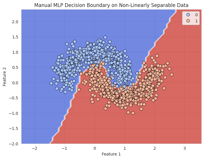
# Plot the decision boundary
x_min, x_max = X[:, 0].min() - 1, X[:, 0].max() + 1
y_min, y_max = X[:, 1].min() - 1, X[:, 1].max() + 1
xx, yy = np.meshgrid(np.arange(x_min, x_max, 0.1), np.arange(y_min, y_max, 0.1))
Z = (sigmoid(np.dot(sigmoid(np.dot(sigmoid(np.dot(np.c_[xx.ravel(), yy.ravel()], weights_1) + bias_1), weights_2) + bias_2), weights_out) + bias_out) > 0.5).astype(int)
Z = Z.reshape(xx.shape)

plt.figure(figsize=(8, 6))
plt.contourf(xx, yy, Z, alpha=0.8, cmap='coolwarm')
sns.scatterplot(x=X[:, 0], y=X[:, 1], hue=y.ravel(), palette="coolwarm", s=60, edgecolor='k')
plt.title("Manual MLP Decision Boundary on Non-Linearly Separable Data")
plt.xlabel("Feature 1")
plt.ylabel("Feature 2")
plt.show()

Epoch 0, Loss: 0.7422
Epoch 100, Loss: 0.2968
Epoch 200, Loss: 0.2715
Epoch 300, Loss: 0.1847
Epoch 400, Loss: 0.1221

Epoch 500, Loss: 0.1006
Epoch 600, Loss: 0.0938
Epoch 700, Loss: 0.1417
Epoch 800, Loss: 0.0788
Epoch 900, Loss: 0.0848

Accuracy: 0.95

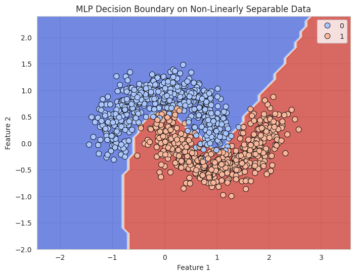
../_images/7f00b10bb98983ba4b565a1be75c6f8af46d1a161c27e409af73010a40aa371c.png

We could have simplified the task by using the MLPClassifier from sklearn to simplify the process (, but without seeing the inner workings of the classifier). For the ones of you intereste, see below.

10.5. Explanation#

Artificial Data Generation: We generate data from two non-linearly separable distributions using the make_moons function, which creates two interleaving half-moon shapes representing the two classes.
Training the MLP: We split the data into training and test sets and train an MLP with two hidden layers (one with 10 neurons and one with 5 neurons).
Evaluation: After training, we evaluate the accuracy of the model on the test data and visualize the decision boundary of the MLP using a contour plot.

10.6. Tuning the MLP#

Hidden Layers: The number and size of hidden layers affect the capacity of the MLP. More layers and neurons allow the model to capture more complex relationships but may lead to overfitting if not properly regularized.
Activation Function: Common activation functions include ReLU, sigmoid, and tanh. The choice of activation function affects how the model learns non-linear patterns.
Learning Rate: Adjusting the learning rate controls how quickly the model updates weights during training. A learning rate that’s too high can lead to instability, while one that’s too low can result in slow convergence.

10.7. A workbench for MLPs#

TensorFlow provides a nice workbench for MLPs, where you can investigate the influence of different selections of input features, architectures, and regularization on performance on different datatypes. Try it out!