Regression

2. Regression#

2.1. General#

The purpose of regression is to model the relationship between a dependent variable (output) and one or more independent variables (inputs). This is one of the most common techniques in statistical modeling, helping us understand and predict the behavior of a dependent variable based on independent variables.

2.1.1. Independent and Dependent Variables#

Independent variable: Denoted as \(\mathbf{x}_i\), these are the input variables or predictors.
Dependent variable: Denoted as \(y_i\), this is the output variable or response we are trying to predict.

2.2. A Linear Regression model#

In a simple case of a linear relationship, we want to find a function that models this relationship. One such model could be linear: \(f(\mathbf{x}_i) = a\mathbf{x}_i + b\), where \(a\) is the slope of the line and \(b\) is the intercept.

We can generalize this model as:

\[f(\mathbf{x}_i') = \mathbf{x}_i'^T \beta\]

Where:

\(\beta = (b, a)^T\) are the model parameters (intercept and slope),
\(\mathbf{x}_i' = (1, \mathbf{x}_i^T)^T\) is the extended input vector including a constant 1 for the intercept,
The goal is to find \(\beta\) that best fits the data.

2.2.1. Residuals#

In regression, the residual for each data point is the difference between the observed value \(y_i\) and the value predicted by the model \(f(\mathbf{x}_i)\). The residual for the \(i\)-th point can be written as:

\[e_i = y_i - f(\mathbf{x}_i)\]

Residuals give us a way to evaluate how well the model fits the data. A smaller residual indicates that the model’s prediction is close to the actual value, while a larger residual suggests a larger error.

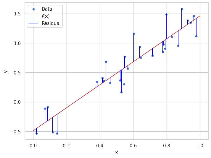
../_images/bf4faa476308457aac82547ca3a249d289398ec650a19eb624e6175fbf9483fd.png

Above is an illustration of the concept of residuals. Given the a model, \(f(\mathbf{x})\), of the data points \(\{(\mathbf{x}_i, y_i)\}_i\), how much of the data “remains to be explained”.

2.2.2. Least Squares Estimation#

To fit a function \(f(\mathbf{x})\) to the data points \(\{(\mathbf{x}_i, y_i)\}_i\), we minimize the sum of squared errors (SSE):

\[\mathcal{l}_{\text{SSE}}=\sum_i^N e_i^2 = \sum_i^N (y_i - f(\mathbf{x}_i) )^2\]

This process is known as least squares. \(\mathcal{l}\) is known as a loss function. The loss is an indication of how well a regression fits the data. Different regression lines will have different losses. By minimizing the loss function, we find the function that best fits the data according to the selected loss function.

If the errors \(e_i\) follow a normal distribution, the maximum likelihood estimation (MLE) is equivalent to least squares minimization, making this approach optimal under these assumptions.

Minimizing SSE is also equivalent to minimizing an even more popular loss function, the Mean Square Error, MSE.

\[\mathcal{l}_{\text{MSE}}=\frac{1}{N}\sum_i^N e_i^2 = \frac{1}{N}\sum_i^N (y_i - f(\mathbf{x}_i) )^2\]

2.2.3. Fit a Linear Model to Data#

A general pattern for machine learning, is the utilization of an optimizer for the minimization of a loss function.

One such method is to manually minimize the loss function, which is the error between the predicted and actual values, using optimization techniques. This approach opens the door to advanced regression models and custom loss functions that aren’t necessarily linear.

Here, we use the scipy.optimize.minimize function to achieve the same linear regression result by explicitly defining a loss function and minimizing it.

from scipy.optimize import minimize
import numpy as np
import seaborn as sns
import matplotlib.pyplot as plt

# Seaborn settings
sns.set(style="whitegrid")

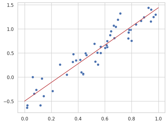
# Generating random data
rng = np.random.RandomState(0) #Here we could give any number a a seed for the random number generator
x = rng.rand(50)
y_linear = 2 * x - 0.5 + 0.2*rng.randn(50)

# Define a generic loss function for both linear and polynomial models
def loss(params, model_function, x, y):
    return np.sum((y - model_function(x, params))**2)

# Define the linear model function
def linear_model(x, params):
    slope, intercept = params
    return slope * x + intercept

# A function searching for a set of parameters that minimize a given loss function over data
def minimize_loss(loss, model, x, y, num_params):
    initial_params = np.random.randn(num_params)
    return minimize(loss, initial_params, args=(model, x, y))

# Minimize the loss function
result_linear = minimize_loss(loss, linear_model, x, y_linear, 2)

# Optimized parameters
slope, intercept = result_linear.x

# Print the optimized slope and intercept
print(f"Optimized slope: {slope}, Optimized intercept: {intercept}")

# Generate prediction line
xfit = np.linspace(0, 1.0, 1000)
yfit_linear = linear_model(xfit, (slope, intercept))

# Plot data and model
sns.scatterplot(x=x, y=y_linear)
plt.plot(xfit, yfit_linear, color='r')
plt.show()

Optimized slope: 1.9385465747718769, Optimized intercept: -0.5014420127199446

../_images/eb5ad5e6aed7d96424fc20c4f88a5e960ceb57e7609bfc7fa95ef62375840bb9.png

In this approach, we use the same underlying concept of minimizing a loss function, but the technique is more flexible, allowing us to extend the method to more advanced models such as polynomial or kernel-based regressions, which we’ll explore in later sections.

The concept of minimizing a loss function provides the foundation for generalizing regression to other types of models and fitting techniques, allowing us to tackle more complex relationships between variables.

2.3. Notes on Optimization#

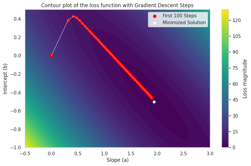
The scipy.optimize.minimize uses a variant of Gradient descent to find an optimal set of parameters (a,b). Gradient Descent is an iterative optimization algorithm used in finding the minimum of a function. Here, we use it for finding the parameters that minimize the loss function.

2.3.1. Concept of Gradient Descent#

The basic idea of gradient descent is to update the parameters in the opposite direction of the gradient of the loss function with respect to the parameters. This is because the gradient points in the direction of the steepest ascent, and we want to go in the opposite direction to find the minimum.

Here is an illustration of how gradient descent to find the optimal \(a\) and \(b\) for our linear regression model. We will also create a contour plot of the loss function as a function of \(a\) and \(b\) to visualize the optimization process.

../_images/78cbf0aa9002472da671f8a6481b689a7be070a8a3f8897296597635d2c86350.png

Optimized slope: 1.9026650146805608, Optimized intercept: -0.4615155987537572

It should be noted that the scipy.optimize.minimize function uses a slightly more advanced version of gradient than illustrated here.

Note

Mathematical Formulation of Gradient Descent

To understand gradient descent mathematically, let’s start with a simple one-dimensional case. Suppose we have a function \(f(\beta)\) and want to find its minimum. The derivative of \(f\) with respect to \(\beta\), denoted as \(f'(\beta)\), gives the slope of the function at any point \(\beta\). Gradient descent updates \(\beta\) iteratively in the opposite direction of \(f'(\beta)\) to move toward the minimum:

\[\beta_{\text{new}} = \beta - \eta f'(\beta)\]

where \(\eta\) is the step size (learning rate), a small positive scalar controlling the step size. This process continues until \(f'(\beta) \approx 0\), indicating that we have reached a local minimum.

Extending to Multiple Dimensions

In higher dimensions, we consider a multivariable function \(L(\boldsymbol{\beta})\), where \(\boldsymbol{\beta} = \begin{bmatrix} \beta_1 \\ \beta_2 \\ \vdots \\ \beta_n \end{bmatrix}\) represents the coefficients of the model in column vector form, and \(L\) is the loss function we aim to minimize. Instead of a single derivative, we use the gradient, denoted \(\nabla L(\boldsymbol{\beta})\), which is a column vector of partial derivatives with respect to each coefficient:

\[\begin{split}\nabla L(\boldsymbol{\beta}) = \begin{bmatrix} \frac{\partial L}{\partial \beta_1} \\ \frac{\partial L}{\partial \beta_2} \\ \vdots \\ \frac{\partial L}{\partial \beta_n} \end{bmatrix}\end{split}\]

Each component \(\frac{\partial L}{\partial \beta_i}\) represents the rate of change of \(L\) with respect to \(\beta_i\). The gradient \(\nabla L(\boldsymbol{\beta})\) points in the direction of the steepest increase of \(L\); therefore, moving in the opposite direction of \(\nabla L(\boldsymbol{\beta})\) decreases \(L\).

The gradient descent update rule for multiple coefficients is:

\[\boldsymbol{\beta}_{\text{new}} = \boldsymbol{\beta} - \eta \nabla L(\boldsymbol{\beta})\]

where \(\eta\) is the step size, determining the update amount at each step.

Applying Gradient Descent to Linear Regression

In our linear regression model, we minimize a loss function, typically the sum of squared errors \(L(a, b)\) for coefficients \(a\) (slope) and \(b\) (intercept). The gradient of \(L\) with respect to \(a\) and \(b\) consists of the partial derivatives \(\frac{\partial L}{\partial a}\) and \(\frac{\partial L}{\partial b}\), which we can express in column vector form as:

\[\begin{split}\nabla L(a, b) = \begin{bmatrix} \frac{\partial L}{\partial b} \\ \frac{\partial L}{\partial a} \end{bmatrix} = \begin{bmatrix} -2 \sum \left( y_i - (a x_i + b) \right) \\ -2 \sum x_i \left( y_i - (a x_i + b) \right) \end{bmatrix}\end{split}\]

The updates for \(a\) and \(b\) are then:

\[\begin{split}\begin{bmatrix} b_{\text{new}} \\ a_{\text{new}} \end{bmatrix} = \begin{bmatrix} b \\ a \end{bmatrix} - \eta \begin{bmatrix} \frac{\partial L}{\partial b} \\ \frac{\partial L}{\partial a} \end{bmatrix}\end{split}\]

With each iteration, \(a\) and \(b\) are adjusted to reduce \(L(a, b)\), bringing us closer to the minimum loss, which corresponds to the optimal coefficients for the model.

2.4. Scikit-learn#

It should be noted that the method described above, by explicitly defining an loss function and minimizing it with a direct call to an optimizer, is selected for explaining something about machine learning, and not the preferd practical approach to e.g. linear regression. Instead linear regression uses an analytical solution to the least squares problem, a well-known method for deriving the optimal parameters.

Instead of thinking too hard on the implementation, we would use a package for the task. Here, scikit-learn is one of the most popular open-source machine learning libraries in Python. It provides simple and efficient tools for data mining and data analysis, making it ideal for academic and industrial applications alike. Built on top of well-established libraries like NumPy, SciPy, and Matplotlib, scikit-learn offers a wide range of machine learning algorithms for both supervised and unsupervised learning tasks.

2.4.1. Key Features:#

Easy to use: scikit-learn’s consistent API and clear documentation make it accessible to beginners.
Wide range of algorithms: It includes support for classification, regression, clustering, dimensionality reduction, and model selection techniques.
Interoperable: scikit-learn integrates seamlessly with other Python libraries like pandas and NumPy, allowing for smooth data handling and preprocessing.

2.4.2. Linear Regression using Scikit-learn.#

The scikit-learn package offers efficient functions for performing linear regression right out of the box. Below is an example where we generate random data following a linear trend, then fit a linear model using the LinearRegression class.

This approach is both fast and highly optimized, making it easy to apply linear regression with minimal setup.

from sklearn.linear_model import LinearRegression

model = LinearRegression(fit_intercept=True)

model.fit(x[:, np.newaxis], y_linear)

xfit = np.linspace(0, 1, 1000)
yfit = model.predict(xfit[:, np.newaxis])

# Scatter plot with seaborn
sns.scatterplot(x=x, y=y_linear)
plt.plot(xfit, yfit, color='r')
plt.show()

2.5. Regression with Kernel Methods#

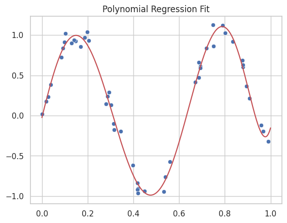
Linear regression is one of the simplest and most widely used models for supervised learning. Now, lets explore how to expand the linear regression model to model non-linear data, by expanding our data into multiple features with kernel functions.

2.5.1. Polynomial Kernels as Basis Functions#

In the previous sections, we explored linear regression and saw that the goal is to minimize a loss function (such as the sum of squared residuals) to obtain the best-fit model. This concept is central to regression tasks, regardless of whether the model is linear or non-linear.

One powerful approach for non-linear regression is to use polynomial basis functions. Polynomial regression can be thought of as applying a kernel transformation to the data by creating higher-order polynomial terms, such as \(x^2\), \(x^3\), and so on. These terms allow us to capture more complex patterns in the data.

For example, instead of fitting a linear model \(y = a x + b\), we can fit a polynomial of degree \(n\), which effectively transforms the input space into a higher-dimensional space where the relationship between \(x\) and \(y\) may be linear, even if the relationship appears non-linear in the original space.

In fact, polynomial kernels can be used to implicitly transform the data without explicitly computing the higher-dimensional features. In kernel-based models like Support Vector Machines (SVM) or kernel ridge regression, a polynomial kernel can be used to fit more complex functions to the data while still employing the same optimization techniques as in linear regression.

import seaborn as sns
import matplotlib.pyplot as plt
import numpy as np

# Seaborn settings
sns.set(style="whitegrid")

# Generating random data
rng = np.random.RandomState(1)
x = rng.rand(50)
y_linear = 2 * x - 3 + 0.2*rng.randn(50)
y_non_linear = np.sin(10.*x) + 0.1 * rng.randn(50)

# Define the polynomial model function
def polynomial_model(x, params, degree=7):
    x_poly = np.vstack([x**i for i in range(degree + 1)]).T
    return np.dot(x_poly, params)


# Optimize the parameters of our model using the same SSE loss function as before 
result_poly = minimize_loss(loss, polynomial_model, x, y_non_linear,8)

poly_params = result_poly.x

# Generate fit lines
yfit_poly = polynomial_model(xfit, poly_params)

sns.scatterplot(x=x, y=y_non_linear)
plt.plot(xfit, yfit_poly, color='r')
plt.title("Polynomial Regression Fit")
plt.show()

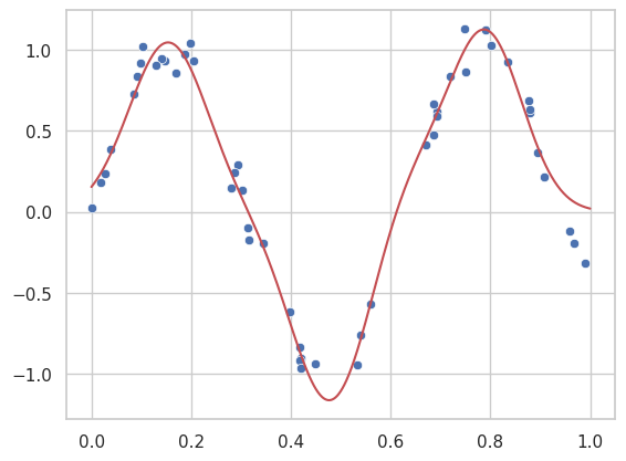
../_images/eb30840ffd428fa47361398190973fad507d639f99eb5901e60224831e3090c3.png

2.5.2. Gaussian Kernels#

We can further extend this concept by introducing other types of kernel functions, such as Gaussian kernels. These kernels, also known as radial basis functions (RBF), allow us to capture localized, non-linear behavior in the data. In essence, Gaussian kernels provide a more flexible model that can handle highly non-linear patterns.

2.5.3. Unifying Loss Minimization Across Models#

What is essential in all these models—whether linear, polynomial, or Gaussian—is that we continue to use the same framework of minimizing a loss function to find the best-fit parameters. The kernel-based approach simply transforms the input space, allowing us to apply non-linear transformations without changing the fundamental concept of minimizing error.

In the next chapter, we will explore more advanced loss functions and regularization techniques, which help control model complexity and prevent overfitting, particularly important in high-dimensional kernel-transformed spaces.

# Define a Gaussian basis function
def gaussian_basis(x, centers, width):
    return np.exp(-0.5 * ((x[:, np.newaxis] - centers[np.newaxis, :]) / width)**2)

# Define the Gaussian model
def gaussian_model(x, params):
    # Split the params into weighths, centers and common width of the bases
    N = len(params)//2
    weights = params[:N]
    centers = params[N:2*N]
    width = params[-1]
    # Calculate the values of each basis for each x 
    basis = gaussian_basis(x, centers, width)
    return np.dot(basis, weights)

N = 15  # Number of Gaussian bases to fit to our data

# Optimize the parameters of our model using the same SSE loss function as before 
result_gaussian = minimize_loss(loss, gaussian_model, x, y_non_linear, N*2+1)
gaussian_params = result_gaussian.x

yfit_gauss = gaussian_model(xfit, gaussian_params)

# Plot the gausian fit
sns.scatterplot(x=x, y=y_non_linear)
plt.plot(xfit, yfit_gauss, color='r')
plt.show()

../_images/ff664af90f0f307d380618c02a82cc3e54f48b9dce391b4e5d9f97656e45404a.png

By focusing on the unified concept of loss minimization, we can see that even complex, non-linear models follow the same principles as basic linear regression—only the structure of the model and the basis functions (kernels) change.