8. Support Vector Machines

8.1. Linear SVMs

Support Vector Machines (SVMs) are powerful tools for classification tasks, and one of the simplest versions is the Linear SVM. A Linear SVM aims to find the optimal line (or hyperplane in higher dimensions) that separates data points into different classes while maximizing the distance between the classes. This distance is called the margin. In this chapter, we’ll explore how Linear SVMs achieve this, using a few examples to help you visualize the concepts.

8.1.1. The Goal of an SVM: Maximum Margin Hyperplane

Imagine we have a set of points that belong to two different classes, represented by the labels +1 and −1. These points, denoted as \((\mathbf{x}_i, y_i)\), where \(y_i\) is either +1 or −1, form our training data. Each \(\mathbf{x}_i\) is a p-dimensional real vector that represents the features of a data point.

The primary goal of an SVM is to find a maximum-margin hyperplane that best divides the data into two classes. The hyperplane should maximize the distance between itself and the nearest points from both classes, which are called support vectors. These support vectors are critical to defining the optimal separating boundary.

8.1.2. Defining a Hyperplane

In a p-dimensional space, a hyperplane can be described by the equation:

\[\mathbf{w}^T \mathbf{x} - b = 0\]

where:

• \(\mathbf{w}\) is the normal vector to the hyperplane, indicating its orientation.

• \(b\) is a parameter that controls the offset of the hyperplane from the origin.

A key objective in Linear SVMs is to find \(\mathbf{w}\) and \(b\) that maximize the margin—the distance between the hyperplane and the closest data points.

8.1.3. Hard-Margin SVM

If the data is perfectly linearly separable (i.e., there exists a hyperplane that separates the classes without any overlap), we can create two parallel hyperplanes, one for each class. The region between these two hyperplanes is called the margin, and the hyperplane exactly in the middle of this margin is called the maximum-margin hyperplane.

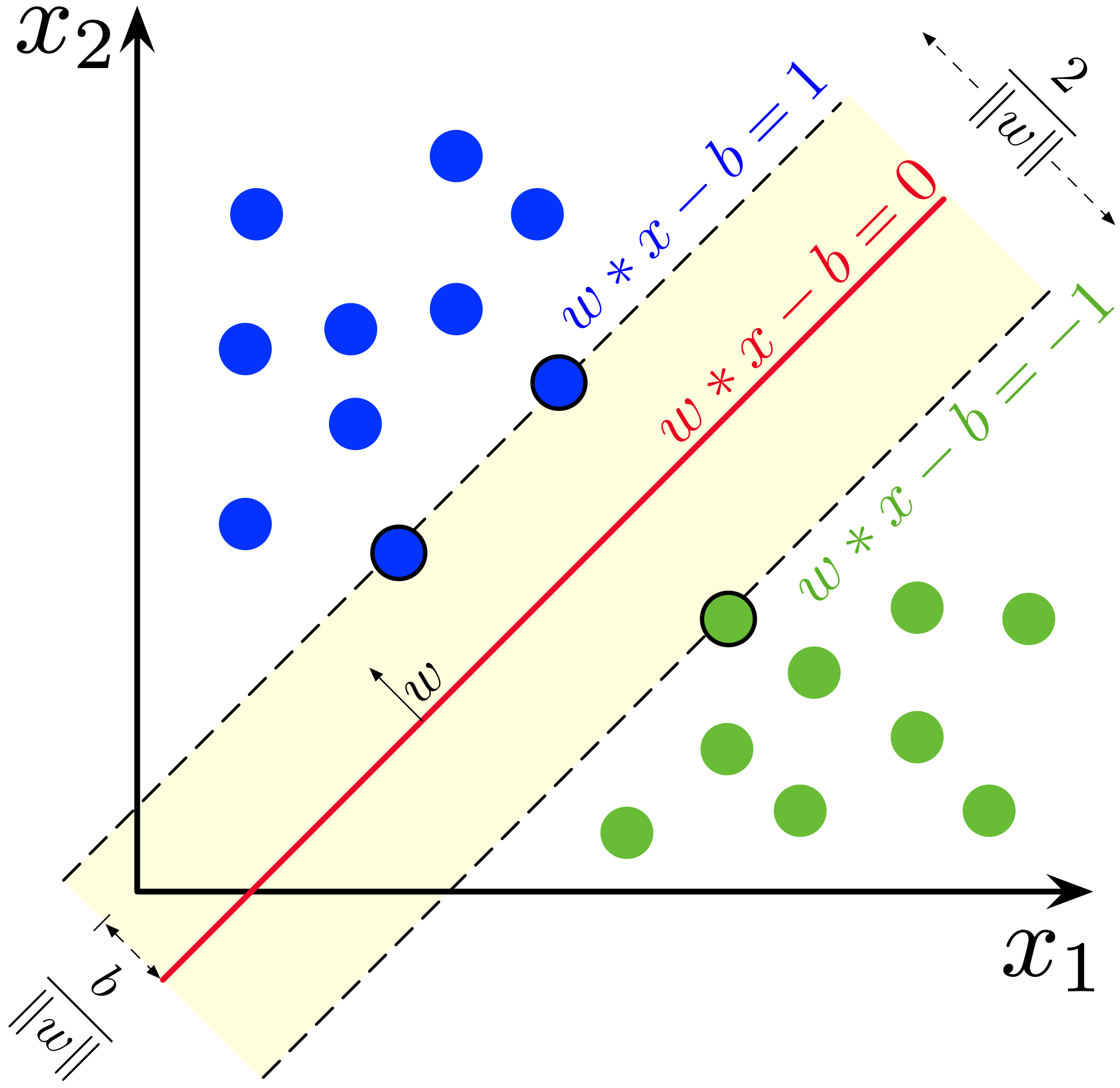
Fig. 8.1 Maximum-margin hyperplane and margins.
Image by Larhmam, CC BY-SA 4.0

The equations for the two parallel hyperplanes are:

\[\mathbf{w}^T \mathbf{x} - b = 1 \quad \text{and} \quad \mathbf{w}^T \mathbf{x} - b = -1\]

These equations indicate that the points on or above one hyperplane belong to class +1, and those on or below the other belong to class −1. The distance between the hyperplanes is given by:

\[\frac{2}{\| \mathbf{w} \|}\]

To maximize this distance, we need to minimize \(\| \mathbf{w} \|\). At the same time, we need to ensure that every point lies on the correct side of the margin, which leads to the following constraint for each data point:

\[y_i (\mathbf{w}^T \mathbf{x}_i - b) \geq 1 \quad \forall i\]

8.1.4. Optimization Problem

The optimization problem for a hard-margin SVM can be formulated as:

\[\min_{\mathbf{w}, b} \frac{1}{2} \| \mathbf{w} \|^2 \quad \text{subject to:} \quad y_i (\mathbf{w}^T \mathbf{x}_i - b) \geq 1 \; \forall i\]

This formulation ensures that we are maximizing the margin while keeping all data points on the correct side of the boundary.

8.1.5. Soft-Margin SVM

In real-world scenarios, data is often not perfectly linearly separable. To handle this, we introduce the concept of a soft margin. Instead of forcing every data point to be on the correct side of the hyperplane, we allow some points to fall inside the margin or even be misclassified. To measure this, we use the hinge loss function:

\[\max(0, 1 - y_i (\mathbf{w}^T \mathbf{x}_i - b))\]

This loss function is zero if the point is correctly classified with enough margin, and increases as the point falls closer to or on the wrong side of the margin.

The goal for a soft-margin SVM is to minimize the following expression:

\[\| \mathbf{w} \|^2 + C \left[ \frac{1}{n} \sum_{i=1}^n \max(0, 1 - y_i (\mathbf{w}^T \mathbf{x}_i - b)) \right]\]

Here, \(C > 0\) is a parameter that controls the trade-off between maximizing the margin and minimizing the classification errors. A larger value of \(C\) puts more emphasis on correctly classifying every point, while a smaller value allows for a wider margin with some misclassifications.

8.1.6. Support Vectors

An important feature of SVMs is that the maximum-margin hyperplane is determined only by the points that lie closest to it—the support vectors. These points are crucial, as they define the boundary of the margin and determine the final classifier. All other points do not directly affect the hyperplane.