19. Autoencoders#
19.1. Introduction#
Autoencoders are a general framework used to learn efficient representations of data, often for dimensionality reduction or feature extraction. They operate by training a model to compress input data into a lower-dimensional representation and then reconstruct the original data from that compressed form. The primary goal of an autoencoder is not merely to copy the input, but rather to discover meaningful patterns and structures that capture the underlying features in a more compact representation.
An autoencoder consists of two main components: the encoder and the decoder. The encoder is responsible for compressing the input into a latent space representation, often called the bottleneck, which is typically of lower dimension than the input. The decoder, in turn, reconstructs the original data from this latent representation. Mathematically, let \(x\) be the input data, the encoder function \(f_{\phi}\) maps \(x\) to a latent vector \(z\), while the decoder function \(g_{\theta}\) reconstructs \(x\) from \(z\), such that:
The model is trained to minimize the reconstruction loss, typically using a loss function like the mean squared error (MSE) between the original input \(x\) and the reconstructed output \(\hat{x}\):
This objective ensures that the latent representation retains as much relevant information about the original data as possible while being compressed. The encoder-decoder architecture can introduce non-linearity through the use of activation functions such as ReLU or sigmoid, making autoencoders capable of capturing more complex relationships than purely linear methods.
Autoencoders have several variations, such as denoising autoencoders, which add noise to the input data during training to make the representation more robust, and variational autoencoders (VAEs), which impose a probabilistic structure on the latent space for generative purposes.
In the next section, we will see how Principal Component Analysis (PCA) can be understood as a simple form of autoencoder, where both the encoder and decoder are linear functions and the latent representation is defined by the principal components. This perspective helps bridge the gap between classical statistical methods and modern approaches to dimensionality reduction.
19.2. PCA as an Autoencoder#
Principal Component Analysis (PCA) can be interpreted as a specific type of autoencoder where the encoder and decoder functions are linear. In PCA, the encoder projects the input data onto a lower-dimensional subspace defined by the principal components, effectively compressing the data while retaining the directions of maximum variance. The decoder then reconstructs the data by projecting back from this subspace to the original space.
To understand why the maximization of the variance in the components is equivalent to minimizing the variance in the residuals, consider the nature of PCA. PCA seeks to find a set of orthogonal directions (principal components) along which the variance of the data is maximized. By capturing the maximum variance in the first few components, the reconstruction error (defined as the difference between the original data and its projection onto these components) is minimized. This is equivalent to saying that PCA minimizes the variance of the residuals, which is the part of the data that cannot be explained by the selected components.
Mathematically, PCA can be expressed using Singular Value Decomposition (SVD), which decomposes the data matrix \(X\) into three matrices: \(U\), \(S\), and \(V^T\), such that:
Here, \(U\) and \(V\) contain the principal components (e.g. your gene-specific and sample-specific effects), and \(S\) is a diagonal matrix of singular values. The first \(k\) columns of \(V\) define the principal components, and by projecting \(X\) onto these components, we obtain the low-dimensional representation. The reconstruction of \(X\) from these \(k\) components can be seen as minimizing the reconstruction error in terms of mean squared error (MSE), making SVD and PCA equivalent to minimizing the MSE in an autoencoder framework.
This perspective provides insight into how PCA is fundamentally related to linear autoencoders: both aim to represent data in a compressed form while preserving as much information as possible, with PCA focusing explicitly on maximizing variance and minimizing reconstruction error.
19.2.1. Implementing Autoencoders with Multilayer Perceptrons (MLPs)#
19.2.1.1. The PyTorch Package#
PyTorch is a popular open-source deep learning framework developed by Facebook’s AI Research lab. It provides a flexible and efficient platform for building and training neural networks, including autoencoders. PyTorch uses a dynamic computation graph, which makes it particularly user-friendly for experimenting with different model architectures, as changes can be made on-the-fly without needing to recompile the entire graph.
PyTorch’s core components include torch.Tensor for handling multi-dimensional data, nn.Module for defining neural network layers and models, and the torch.optim package for optimizing models. These features make it straightforward to implement and train complex architectures, such as autoencoders, with relatively few lines of code.
Autoencoders can be implemented using Multilayer Perceptrons (MLPs), which are neural networks composed of multiple layers of interconnected nodes. In an MLP-based autoencoder, both the encoder and decoder are typically represented as feedforward neural networks with one or more hidden layers.
Note that there are several other tensor packages available with similar functionality as torch, e.g. tensorflow and JAX.
19.2.1.2. Implementation#
To implement an autoencoder with an MLP, we start by defining the architecture. The encoder consists of a series of connected layers that reduce the dimensionality of the input data until reaching the bottleneck layer, which represents the latent space. The decoder then consists of a series of layers that expand the latent representation back to the original input dimension.
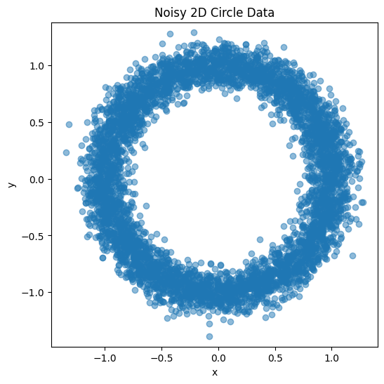
A simple MLP-based autoencoder can be implemented in Python using popular deep learning libraries like TensorFlow or PyTorch. Below is an example implementation using PyTorch. As a test case, lets consider synthetic data with a certain structure, 2D data from a “noisy” circle, that we scramble by projecting it into a 10 dimensional space. Could we train an encoder that in its latent representation capture the original structure of the data?
Steps Summary of the code:
Generate 2D Circle Data with Noise:
Use numpy to create 2D points on a noisy circle.
Visualize the generated data using matplotlib.
Project Data into 10D Space:
Apply a random linear transformation to the 2D data to create 10-dimensional representations. We do this to hide the actual structure of the data for the autoencoder. Our hope is that the encoder will learn to reverse this random transformation.
Define and Train the Autoencoder:
The autoencoder consists of an encoder that compresses 10D data into a 2D latent space and a decoder that reconstructs it back to the original 10D.
Train the autoencoder using a Mean Squared Error loss to reconstruct the original high-dimensional data.
Plot the Latent Space Embeddings:
After training, visualize the latent representations to see how well the model compresses the data back into 2D.
import torch
import torch.nn as nn
import torch.optim as optim
import numpy as np
import matplotlib.pyplot as plt
from torch.utils.data import DataLoader, TensorDataset

# Step 1: Generate 2D points on a circle with noise
n_samples = 5000
noise_level = 0.1
np.random.seed(42)

theta = 2 * np.pi * np.random.rand(n_samples)
x = np.cos(theta) + noise_level * np.random.randn(n_samples)
y = np.sin(theta) + noise_level * np.random.randn(n_samples)

# Plot the original noisy circle data
plt.figure(figsize=(6, 6))
plt.scatter(x, y, alpha=0.5)
plt.title("Noisy 2D Circle Data")
plt.xlabel("x")
plt.ylabel("y")
plt.axis('equal')
plt.show()

# Step 2: Project the 2D data to a 10-dimensional space
points_2d = np.vstack((x, y)).T
projection_matrix = np.random.randn(2, 10)
high_dim_points = points_2d @ projection_matrix

# Convert to PyTorch tensors
high_dim_points = torch.tensor(high_dim_points, dtype=torch.float32)
dataset = TensorDataset(high_dim_points)
dataloader = DataLoader(dataset, batch_size=32, shuffle=True)

# Step 3: Define the Autoencoder with a 2D latent space
class Autoencoder(nn.Module):
    def __init__(self, input_dim, hidden_dim, latent_dim):
        super(Autoencoder, self).__init__()
        # Encoder network
        self.encoder = nn.Sequential(
            nn.Linear(input_dim, hidden_dim),
            nn.ReLU(),
            nn.Linear(hidden_dim, latent_dim)
        )
        # Decoder network
        self.decoder = nn.Sequential(
            nn.Linear(latent_dim, hidden_dim),
            nn.ReLU(),
            nn.Linear(hidden_dim, input_dim)
        )

    def forward(self, x):
        z = self.encoder(x)
        reconstructed = self.decoder(z)
        return z, reconstructed

# Set up model, loss function, and optimizer
input_dim = 10
hidden_dim = 6
latent_dim = 2
autoencoder = Autoencoder(input_dim, hidden_dim, latent_dim)

criterion = nn.MSELoss()
optimizer = optim.Adam(autoencoder.parameters(), lr=1e-3)

# Step 4: Train the autoencoder
num_epochs = 50
for epoch in range(num_epochs):
    for data in dataloader:
        inputs, = data

        # Forward pass
        latent, outputs = autoencoder(inputs)
        loss = criterion(outputs, inputs)

        # Backward pass
        optimizer.zero_grad()
        loss.backward()
        optimizer.step()

    if (epoch + 1) % 10 == 0:
        print(f'Epoch [{epoch+1}/{num_epochs}], Loss: {loss.item():.4f}')

# Step 5: Plot the latent space embeddings
all_inputs = high_dim_points
with torch.no_grad():
    latent_embeddings, _ = autoencoder(all_inputs)

latent_embeddings = latent_embeddings.numpy()

plt.figure(figsize=(6, 6))
plt.scatter(latent_embeddings[:, 0], latent_embeddings[:, 1], alpha=0.5)
plt.title("Latent Space Embeddings")
plt.xlabel("Latent Dimension 1")
plt.ylabel("Latent Dimension 2")
plt.axis('equal')
plt.show()
Epoch [10/50], Loss: 0.0034
Epoch [20/50], Loss: 0.0020
Epoch [30/50], Loss: 0.0009
Epoch [40/50], Loss: 0.0003
Epoch [50/50], Loss: 0.0001
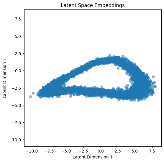
In this implementation, the Autoencoder class defines both the encoder and decoder as sequential networks. The encoder compresses the input to a latent dimension, while the decoder reconstructs the input from the latent representation. The network is trained by minimizing the mean squared error (MSE) between the input and the reconstructed output.
The activation functions used in the encoder and decoder introduce non-linearity, enabling the autoencoder to learn more complex mappings than PCA. The ReLU activation is commonly used in the hidden layers, while the output layer uses a Sigmoid activation to ensure the reconstructed values are in a specific range (e.g., [0, 1] for normalized data).
MLP-based autoencoders are a powerful tool for learning non-linear representations of data, which makes them well-suited for tasks involving complex, high-dimensional datasets. By stacking multiple hidden layers, the autoencoder can capture increasingly abstract features, enabling effective dimensionality reduction and feature extraction.
19.3. Variational Autoencoders (VAEs)#
Variational autoencoders (VAEs) are an extension of autoencoders designed to be used for generative purposes. In order to generate new data points from the latent space, it is important that the latent space is structured in a regular and continuous manner. To achieve this, VAEs introduce explicit regularization during the training process, which ensures that the latent space has desirable properties that facilitate generative tasks.
The decoder of the VAE acts as a generative model, which means that we can use it to generate new data points by sampling from the latent space. By sampling from the standard normal distribution that the latent space is regularized to follow, we can feed these samples into the decoder to produce entirely new examples. This capability makes VAEs powerful tools for generating new, diverse data points that are consistent with the patterns learned from the training data.
Similar to standard autoencoders, VAEs consist of an encoder and a decoder, and the model is trained to minimize the reconstruction error between the input and the reconstructed output. However, the key difference is that, instead of encoding the input as a single point in the latent space, VAEs encode the input as a probability distribution over the latent space. This modification helps introduce a regularization mechanism that ensures the latent space is organized in a way that allows for effective data generation.
To make this process differentiable and enable backpropagation, VAEs use a technique called the reparameterization trick. Instead of sampling directly from the latent distribution, the reparameterization trick involves expressing the latent variable as a function of the mean and standard deviation. We replace the sampling from the latent variable \(z \sim N(\mu, \sigma)\) with a deterministic transformation \(z = \mu + a \sigma\), where \(a \sim N(0, 1)\). This transformation ensures that the gradient can flow through the sampling operation, allowing us to perform backpropagation effectively.
In VAEs, the training process is as follows:
The input is encoded as a distribution over the latent space.
A point is sampled from the latent space using the encoded distribution.
The sampled point is passed through the decoder to reconstruct the original input.
The reconstruction error is computed and backpropagated through the network.
In practice, the encoded distributions are typically Gaussian, and the encoder outputs the mean and covariance matrix for these Gaussians. This allows the latent space to be described probabilistically, providing a natural way to introduce regularity. The encoder is trained to ensure that the returned distributions are close to a standard normal distribution, with a mean of zero and unit variance, ensuring that the latent space is both continuous and complete.
The loss function for training a VAE has two components:
Reconstruction Term: This term ensures that the reconstructed output is as similar as possible to the original input, thereby minimizing the reconstruction error.
Regularization Term: This term, known as the Kullback-Leibler (KL) divergence, ensures that the distributions returned by the encoder are close to a standard normal distribution. The KL divergence measures the difference between the encoded distribution and the standard Gaussian, encouraging the latent space to be organized in a way that allows for meaningful generative capabilities.
The regularization of the latent space helps achieve two key properties:
Continuity: Close points in the latent space should produce similar outputs when decoded, which ensures a smooth transition in the generated data.
Completeness: Every point in the latent space should produce a meaningful output when decoded, allowing the model to generate diverse but realistic data points.
Without the regularization term, the model could overfit and behave like a standard autoencoder, where the latent distributions become either too narrow (leading to punctual distributions) or too far apart (leading to gaps in the latent space). By enforcing the latent space to resemble a standard normal distribution, VAEs prevent overfitting and ensure that the latent space is well-structured for generation purposes.
19.3.1. Intuitions about the Regularization of VAEs#
The regularity expected from the latent space of a variational autoencoder is crucial to making the generative process effective. This regularity can be understood through two main properties listed above (Continuity and Completeness.) A key difference between a regular and an irregular latent space lies in the ability to satisfy these properties. The fact that VAEs encode inputs as distributions rather than single points is important but not sufficient on its own to ensure continuity and completeness. Without well-defined regularization, the model may ignore the distributional encoding and behave similarly to a standard autoencoder, which could lead to overfitting. This overfitting could occur if the encoder returns distributions with very small variances (effectively collapsing to single points) or if the means of the distributions are very far apart, leading to discontinuities in the latent space.
To address these issues, VAEs employ a regularization term that controls both the covariance matrix and the mean of the latent distributions returned by the encoder. In practice, this regularization is implemented by encouraging the encoded distributions to be close to a standard normal distribution (mean zero and unit variance). By doing so:
The covariance matrices are encouraged to be close to the identity matrix, which prevents the distributions from collapsing into single points and ensures that the encoded points have some spread.
The means are encouraged to be close to zero, preventing the distributions from being too far apart and ensuring that the latent space is densely populated and well-connected.
This type of regularization results in a latent space that has desirable generative properties. It helps prevent the model from placing data points too far apart, thus encouraging overlap in the latent representations, which is critical for achieving both continuity and completeness. The trade-off between the reconstruction loss and the KL divergence ensures that the model learns a latent space that balances reconstruction quality with a well-regularized structure.
19.3.2. Creating a Gradient in the Latent Space#
The regularization of the latent space through the KL divergence creates a form of continuity that can be thought of as a “gradient” across the latent space. For example, if two encoded distributions originate from two different training samples, a point in the latent space that lies midway between their means should ideally decode into something that represents a blend of those two samples. This smooth transition across the latent space allows for meaningful interpolation, where points between different data clusters produce intermediate, plausible outputs.
This property of creating gradients across the latent space is one of the reasons why VAEs are powerful generative models. By ensuring that points in the latent space correspond to smooth changes in the output, VAEs enable the generation of new, diverse samples that maintain a clear relationship with the training data. It is the balance between continuity and completeness, enforced by regularization, that allows VAEs to create new content effectively.
19.3.3. Example Implementation of a VAE#
Here, we provide an example implementation of a Variational Autoencoder (VAE) using the same synthetic data that we used for the autoencoder. In this example, we generate 2D points on a noisy circle, project them to a higher-dimensional space, and train the VAE to encode and decode the data effectively.
import torch
import torch.nn as nn
import torch.optim as optim
import numpy as np
from torch.utils.data import DataLoader, TensorDataset
import matplotlib.pyplot as plt

# Generate 2D points on a circle with noise
n_samples = 5000
noise_level = 0.1
np.random.seed(42)

theta = 2 * np.pi * np.random.rand(n_samples)
x = np.cos(theta) + noise_level * np.random.randn(n_samples)
y = np.sin(theta) + noise_level * np.random.randn(n_samples)

# Project to higher dimensions (e.g., 10D) using a random linear transformation
points_2d = np.vstack((x, y)).T
projection_matrix = np.random.randn(2, 10)
high_dim_points = points_2d @ projection_matrix

# Convert to PyTorch tensors
high_dim_points = torch.tensor(high_dim_points, dtype=torch.float32)
dataset = TensorDataset(high_dim_points)
dataloader = DataLoader(dataset, batch_size=32, shuffle=True)

# Define the VAE model
class VAE(nn.Module):
    def __init__(self, input_dim, hidden_dim, latent_dim):
        super(VAE, self).__init__()
        # Encoder
        self.fc1 = nn.Linear(input_dim, hidden_dim)
        self.fc21 = nn.Linear(hidden_dim, latent_dim)  # Mean of the latent distribution
        self.fc22 = nn.Linear(hidden_dim, latent_dim)  # Log variance of the latent distribution
        # Decoder
        self.fc3 = nn.Linear(latent_dim, hidden_dim)
        self.fc4 = nn.Linear(hidden_dim, input_dim)

    def encode(self, x):
        h1 = torch.relu(self.fc1(x))
        return self.fc21(h1), self.fc22(h1)

    def reparameterize(self, mu, logvar):
        std = torch.exp(0.5 * logvar)
        eps = torch.randn_like(std)
        return mu + eps * std

    def decode(self, z):
        h3 = torch.relu(self.fc3(z))
        return torch.sigmoid(self.fc4(h3))

    def forward(self, x):
        mu, logvar = self.encode(x)
        z = self.reparameterize(mu, logvar)
        return self.decode(z), mu, logvar

# Set up model, loss function, and optimizer
input_dim = 10
hidden_dim = 6
latent_dim = 2
vae = VAE(input_dim, hidden_dim, latent_dim)

optimizer = optim.Adam(vae.parameters(), lr=1e-3)

# Define the loss function
def loss_function(recon_x, x, mu, logvar):
    BCE = nn.functional.mse_loss(recon_x, x, reduction='sum')
    # KL Divergence
    KLD = -0.5 * torch.sum(1 + logvar - mu.pow(2) - logvar.exp())
    return BCE + KLD

# Training loop
num_epochs = 50
for epoch in range(num_epochs):
    vae.train()
    train_loss = 0
    for data in dataloader:
        inputs, = data
        optimizer.zero_grad()
        recon_batch, mu, logvar = vae(inputs)
        loss = loss_function(recon_batch, inputs, mu, logvar)
        loss.backward()
        train_loss += loss.item()
        optimizer.step()

    # print(f'Epoch [{epoch+1}/{num_epochs}], Loss: {train_loss / len(dataloader.dataset):.4f}')

# Plot the latent space embeddings
vae.eval()
with torch.no_grad():
    mu, _ = vae.encode(high_dim_points)
    latent_embeddings = mu.numpy()

plt.figure(figsize=(6, 6))
plt.scatter(latent_embeddings[:, 0], latent_embeddings[:, 1], alpha=0.5)
plt.title("Latent Space Embeddings of VAE")
plt.xlabel("Latent Dimension 1")
plt.ylabel("Latent Dimension 2")
plt.axis('equal')
plt.show()
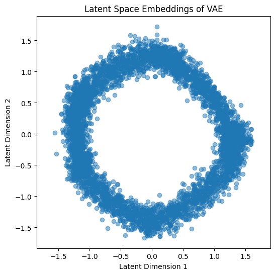
In this implementation, the VAE consists of an encoder that outputs the mean and log variance of the latent distribution, a reparameterization trick to sample from this distribution, and a decoder to reconstruct the input. The loss function includes both a reconstruction term (mean squared error) and a KL divergence term to ensure the latent space is well-regularized. After training, the latent space embeddings are plotted to visualize the learned structure.