15. Unsupervised Machine Learning#
15.1. Introduction#
Unsupervised machine learning aims to learn patterns from data without predefined labels. Specifically, the goal is to learn a function \(f(x)\) from the dataset \(D = \{\mathbf{x}_i\}\) by optimizing an objective function \(g(D, f)\), or by simply partitioning the dataset \(D\). This chapter provides an overview of clustering methods, which are a core part of unsupervised machine learning.
15.2. Clustering#
Clustering is a technique used to partition data into distinct groups, where data points in the same group share similar characteristics. Clustering can be broadly categorized into hard clustering and soft (fuzzy) clustering.
Hard Clustering: In hard clustering, each data point is assigned to a single cluster. This means that each data point belongs exclusively to one group.
Soft (Fuzzy) Clustering: In soft clustering, a data point can belong to multiple clusters with different probabilities. This allows for a more nuanced assignment, where data points can have partial membership across clusters.
15.3. k-Means Clustering#
One of the most common clustering algorithms is k-Means. It is a hard clustering algorithm that aims to partition the dataset into \(k\) clusters by iteratively refining the cluster assignments.
15.3.1. Algorithm Overview#
Cluster Centers: The cluster center \(\mathbf{m}_i\) is defined as the arithmetic mean of all the data points belonging to the cluster.
Distance Metric: Typically, the distance metric used is Euclidean distance, defined as \(||\mathbf{x}_p - \mathbf{m}_i||\).
Cluster Assignment: Each data point is assigned to the nearest cluster center:
\[S_i^{(t)} = \{\mathbf{x}_p: ||\mathbf{x}_p - \mathbf{m}_i^{(t)}||^2 \le ||\mathbf{x}_p - \mathbf{m}_j^{(t)}||^2 \; \forall j \}\]Recalculation of Cluster Centers: The cluster centers are recalculated based on the new assignments:
\[\mathbf{m}_i^{(t+1)} = \frac{1}{|S_i^{(t)}|} \sum_{\mathbf{x}_j \in S_i^{(t)}} \mathbf{x}_j\]
These steps are repeated until the cluster centers converge.
15.3.2. Illustrations of k-Means#
To better understand how the k-Means algorithm works, let’s consider the following visualization steps:
import numpy as np
from sklearn.metrics import pairwise_distances_argmin
from sklearn.datasets import make_blobs
import seaborn as sns
import matplotlib.pyplot as plt

# Generate sample data
X, y_true = make_blobs(n_samples=300, centers=5, cluster_std=0.60, random_state=1)

# Function to plot data points with cluster centers
def plot_kmeans_step(ax, X, centers, labels=None, step_title=""):
    if labels is not None:
        ax.scatter(X[:, 0], X[:, 1], c=labels, s=50, cmap='plasma', label='Data Points')
    else:
        ax.scatter(X[:, 0], X[:, 1], color='gray', s=50, alpha=0.6, label='Data Points')
    sns.scatterplot(x=centers[:, 0], y=centers[:, 1], color='black', s=200, alpha=0.5, ax=ax, label='Cluster Centers')
    ax.set_title(step_title)

# Initialize the plot with a 4x2 grid (4 steps per column for E and M steps)
fig, axes = plt.subplots(4, 2, figsize=(12, 16))
fig.tight_layout(pad=5)

# Step 1: Initial Random Cluster Centers
rng = np.random.RandomState(1)
i = rng.permutation(X.shape[0])[:5]
centers = X[i]
plot_kmeans_step(axes[0, 1], X, centers, step_title="Initial Random Cluster Centers")

# Step 2: First E-Step (assign points to the nearest cluster center)
labels = pairwise_distances_argmin(X, centers)
plot_kmeans_step(axes[1, 0], X, centers, labels, "First E-Step: Assign Points to Nearest Cluster")

# Step 3: First M-Step (recalculate cluster centers)
centers = np.array([X[labels == i].mean(axis=0) for i in range(len(centers))])
plot_kmeans_step(axes[1, 1], X, centers, labels, step_title="First M-Step: Recalculate Cluster Centers")

# Step 4: Second E-Step (assign points to the nearest cluster center)
labels = pairwise_distances_argmin(X, centers)
plot_kmeans_step(axes[2, 0], X, centers, labels, "Second E-Step: Assign Points to Nearest Cluster")

# Step 5: Second M-Step (recalculate cluster centers)
centers = np.array([X[labels == i].mean(axis=0) for i in range(len(centers))])
plot_kmeans_step(axes[2, 1], X, centers, labels, step_title="Second M-Step: Recalculate Cluster Centers")

# Step 6: Third E-Step (assign points to the nearest cluster center)
labels = pairwise_distances_argmin(X, centers)
plot_kmeans_step(axes[3, 0], X, centers, labels, "Third E-Step: Assign Points to Nearest Cluster")

# Step 7: Third M-Step (recalculate cluster centers)
centers = np.array([X[labels == i].mean(axis=0) for i in range(len(centers))])
plot_kmeans_step(axes[3, 1], X, centers, labels, step_title="Third M-Step: Recalculate Cluster Centers")

plt.show()
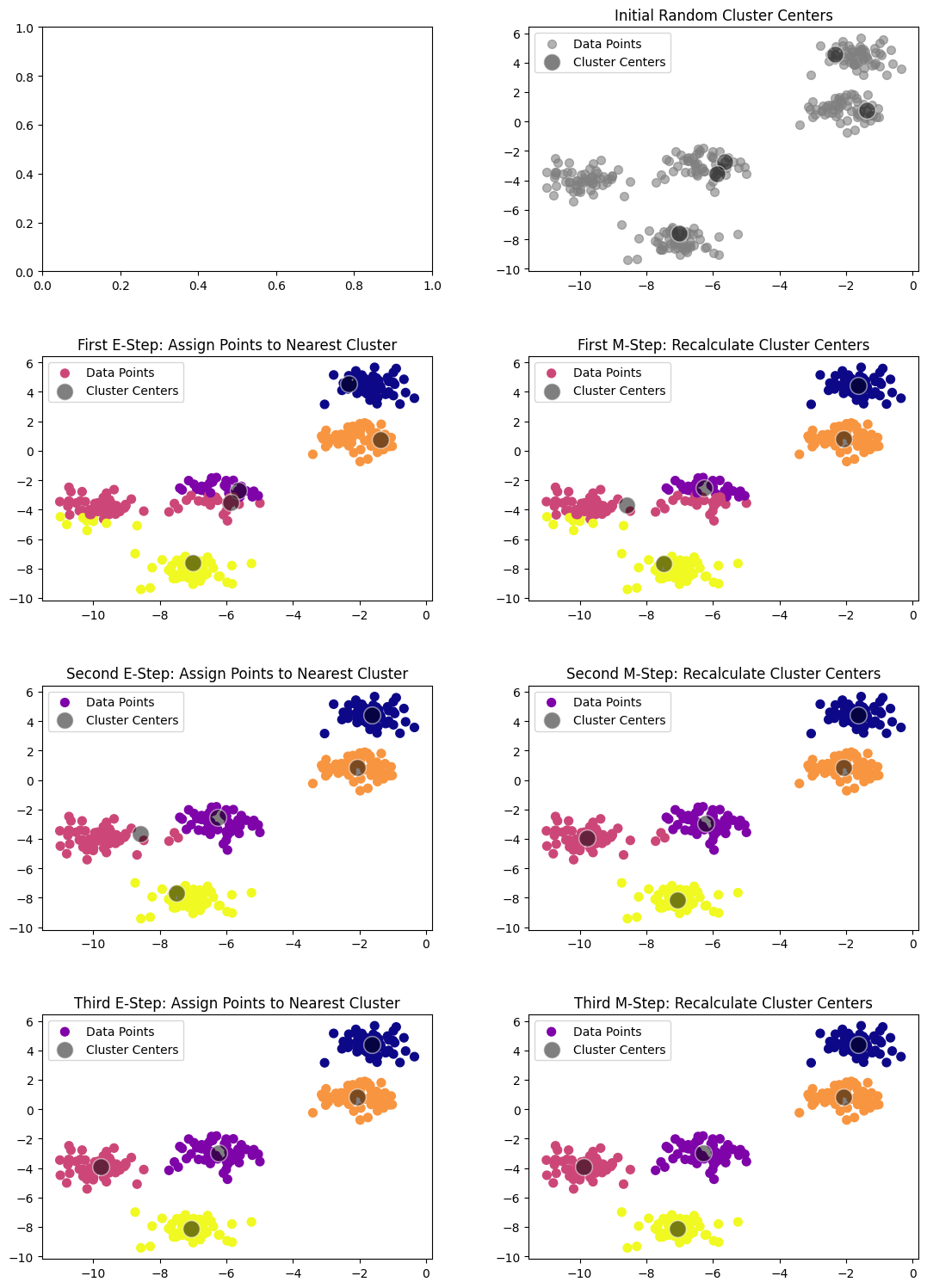
The algorithm automatically assigns the points to clusters, and we can see that it closely matches what we would expect by visual inspection.
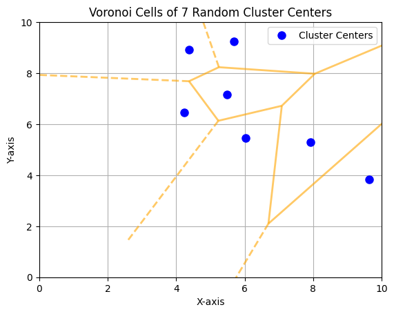
15.3.3. Voronoi Cells and k-Means Clustering#
The k-means clusters form Voronoi cells. In the context of k-means, Voronoi cells represent the regions of influence for each cluster center. Each point in a Voronoi cell is closer to its assigned cluster center than to any other cluster center.
In two dimensions, the Voronoi diagram offers an intuitive way to observe how the space is divided based on the distance to each cluster center. Below, we provide a Python script that visualize the Voronoi cells generated by 7 randomly positioned cluster centers in a 2-dimensional space.
import numpy as np
import matplotlib.pyplot as plt
from scipy.spatial import Voronoi, voronoi_plot_2d

# Generate 7 random cluster centers in 2D space
np.random.seed(0)  # For reproducibility
cluster_centers = np.random.rand(7, 2) * 10

# Compute Voronoi diagram
vor = Voronoi(cluster_centers)

# Plot Voronoi diagram
fig, ax = plt.subplots()
voronoi_plot_2d(vor, ax=ax, show_vertices=False, line_colors='orange', line_width=2, line_alpha=0.6, point_size=10)

# Plot cluster centers
ax.plot(cluster_centers[:, 0], cluster_centers[:, 1], 'bo', markersize=8, label='Cluster Centers')

# Add labels and title
ax.set_title('Voronoi Cells of 7 Random Cluster Centers')
ax.set_xlabel('X-axis')
ax.set_ylabel('Y-axis')
ax.legend()
plt.xlim(0, 10)
plt.ylim(0, 10)
plt.grid()
plt.show()
15.3.4. Drawbacks of k-Means#
The k-Means algorithm is simple and effective, but it has some drawbacks:
Initialization Sensitivity: The algorithm’s result can be highly dependent on the initial choice of cluster centers. Poor initialization may lead to suboptimal clustering, as k-Means may converge to a local minimum. For example, using a different random seed can lead to different cluster assignments.
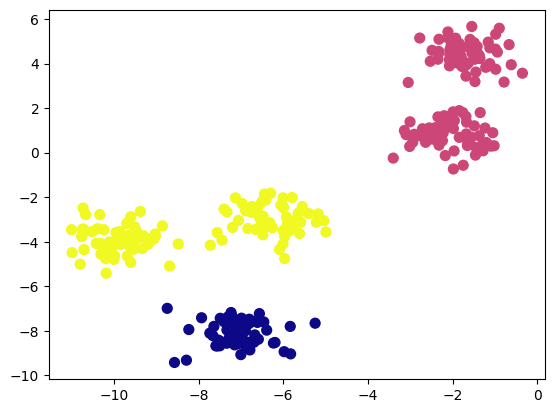
Predefined Number of Clusters: k-Means requires specifying the number of clusters beforehand. For example, if we set the number of clusters to three instead of five, the algorithm will still proceed, but the result may not be meaningful.
from sklearn.cluster import KMeans

labels = KMeans(3, random_state=0).fit_predict(X)
plt.scatter(X[:, 0], X[:, 1], c=labels, s=50, cmap='plasma');
plt.show()
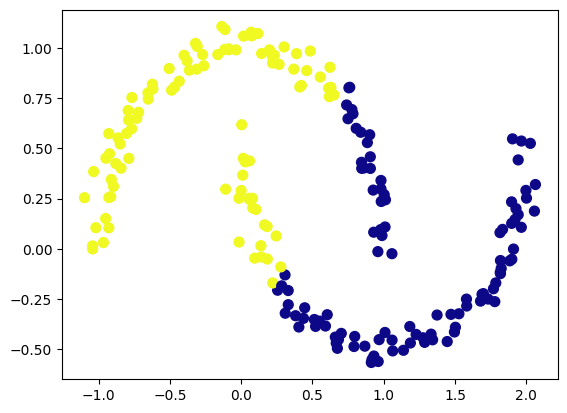
Linear Cluster Boundaries: The k-Means algorithm assumes that clusters are spherical and separated by linear boundaries. It struggles with complex geometries. Consider the following dataset with two crescent-shaped clusters:
from sklearn.datasets import make_moons

X, y = make_moons(200, noise=.05, random_state=42)
labels = KMeans(2, random_state=0).fit_predict(X)
plt.scatter(X[:, 0], X[:, 1], c=labels, s=50, cmap='plasma');
plt.show()
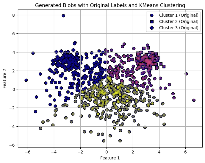
Differences in euclidian size: K-Means assumes that the cluster sizes, in terms of euclidian distance to its borders, are fairly similar for all clusters. Here is an example of three “Mikey Mouse” shaped cludsters, where k-means seems to have a hard time allocating cluster boarders correct.
# Parameters for the blobs
n_samples = [600, 100, 100]
centers = [(0, 0), (3, 3), (-3, 3)]  # Center coordinates
cluster_std = [2., 0.5, 0.5]  # Standard deviations for each blob

# Generate blobs
X, y = make_blobs(n_samples=n_samples, centers=centers, cluster_std=cluster_std, random_state=1)

labels = KMeans(3, random_state=0).fit_predict(X)
# Define markers for the original labels
markers = ['o', 's', 'D']  # Circle, square, and diamond markers for each blob

# Plot with original labels using different marker types
plt.figure(figsize=(8, 6))
for i in range(3):
    plt.scatter(X[y == i, 0], X[y == i, 1], c=[i]*len(X[y == i]),
                label=f"Cluster {i+1} (Original)", marker=markers[i], edgecolor='k', s=50, cmap='plasma')

# Overlay KMeans labels as color-coded dots without specific marker shapes
plt.scatter(X[:, 0], X[:, 1], c=labels, s=20, cmap='plasma', alpha=0.4)
plt.title("Generated Blobs with Original Labels and KMeans Clustering")
plt.xlabel("Feature 1")
plt.ylabel("Feature 2")
plt.legend(loc='upper right')
plt.grid(True)
plt.show()
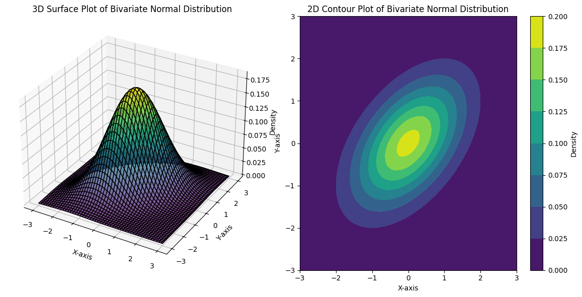
15.4. Multivariate Normal Distribution#
A multivariate normal distribution, also known as a multinormal distribution, is a generalization of the one-dimensional normal distribution to multiple dimensions.
15.4.1. Definition#
A multivariate normal distribution is characterized by a vector of mean values (\(\boldsymbol{\mu}\)) and a covariance matrix (\(\boldsymbol{\Sigma}\)). It describes the joint distribution of a set of random variables, each of which has a univariate normal distribution, but with the potential for covariance between them, allowing for dependencies. Mathematically, if \(\mathbf{X}\) is a random vector \((X_1, X_2, \dots, X_n)\) following a multivariate normal distribution, its probability density function is given by:
where:
\(\mathbf{x}\) is a real \(k\)-dimensional vector,
\(\boldsymbol{\mu}\) is the mean vector,
\(\boldsymbol{\Sigma}\) is the \(k \times k\) covariance matrix,
\(k\) is the number of dimensions (variables),
\(|\boldsymbol{\Sigma}|\) is the determinant of the covariance matrix.
The multivariate normal distribution is fundamental to Gaussian Mixture Models and provides a natural way to model the clusters in high-dimensional data.
15.5. Gaussian Mixture Models (GMM)#
Gaussian Mixture Models (GMMs) provide a probabilistic approach to clustering and are an example of soft clustering. GMMs assume that the data is generated from a mixture of several Gaussian distributions, each representing a cluster. This makes GMMs extremely flexible in modeling complex, multi-modal data distributions that a single Gaussian distribution cannot capture adequately.
15.5.1. Mathematical Formulation#
We model the our full data set as being generated from a mixture of \(K\) Gaussian components. Each of the components being a MultiNormal distribution, \(\mathcal{N}(\mathbf{x}|\mu_k, \Sigma_k)\), with its own mean, \(\mu_k\), and covariance matrix, \(\Sigma_k\) and each component having a mixing coefficient, \(P_k\) that represents the proportion of data points that belong to that component. The probability density function of a GMM with \(K\) components is given by:
15.5.2. EM Algorithm for GM Steps#
Unlike k-Means, GMM provides a soft clustering where each point is assigned a probability of belonging to each cluster.
Here is a detailed description of the Gaussian Mixture Models (GMM) algorithm with the mathematics you provided, outlining its steps:
Initialization:
Define the number of clusters, \( K \).
Initialize the parameters:
Means \( \mu_k \) for each component.
Covariance matrices \( \Sigma_k \) for each component.
Mixing coefficients \( P_k \), such that \( \sum_{k=1}^K P_k = 1 \).
Expectation Step (E-Step):
Compute the probability that a data point \( \mathbf{x}_n \) belongs to cluster \( k \), called the responsibility \( \gamma_{nk} \):
\[\gamma_{nk} = \frac{P_k \mathcal{N}(\mathbf{x}_n | \mu_k, \Sigma_k)}{\sum_{j=1}^K P_j \mathcal{N}(\mathbf{x}_n | \mu_j, \Sigma_j)} \]where:
\( \mathcal{N}(\mathbf{x}_n | \mu_k, \Sigma_k) \) is the Gaussian probability density function:
\[\mathcal{N}(\mathbf{x}_n | \mu_k, \Sigma_k) = \frac{1}{\sqrt{(2\pi)^d |\Sigma_k|}} \exp\left( -\frac{1}{2} (\mathbf{x}_n - \mu_k)^T \Sigma_k^{-1} (\mathbf{x}_n - \mu_k) \right)\]Maximization Step (M-Step):
Recalculate the parameters based on the responsibilities \( \gamma_{nk} \):
Effective number of points in cluster \( k \):
\[N_k = \sum_{n=1}^N \gamma_{nk}\]Updated cluster means:
\[\mu_k^{\text{new}} = \frac{1}{N_k} \sum_{n=1}^N \gamma_{nk} \mathbf{x}_n\]Updated covariance matrices:
\[\Sigma_k^{\text{new}} = \frac{1}{N_k} \sum_{n=1}^N \gamma_{nk} (\mathbf{x}_n - \mu_k^{\text{new}})(\mathbf{x}_n - \mu_k^{\text{new}})^T\]Updated mixing coefficients:
\[P_k^{\text{new}} = \frac{N_k}{N}\]
Log-Likelihood Calculation:
Evaluate the log-likelihood of the data given the current model parameters:
\[\ln \Pr(\mathbf{X} | \boldsymbol{\mu}, \boldsymbol{\Sigma}, \mathbf{P}) = \sum_{n=1}^N \ln \left( \sum_{k=1}^K P_k \mathcal{N}(\mathbf{x}_n | \mu_k, \Sigma_k) \right)\]Convergence Check:
Repeat the E and M steps until convergence, which occurs when the log-likelihood no longer increases or the parameter updates become negligible.
15.5.3. Illustrations of GMM#
To understand GMM better, let’s consider the following visualizations.
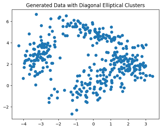
Here is a set of random datapoints generated from distributions where we introduced co-variation between the features.
import numpy as np
import matplotlib.pyplot as plt
from sklearn.mixture import GaussianMixture
from matplotlib.patches import Ellipse

# Function to generate diagonal blobs with custom shapes
def generate_diagonal_blobs(means, covariances, n_samples):
    X = []
    y = []
    for i, (mean, cov) in enumerate(zip(means, covariances)):
        # Generate points for each cluster with given mean and covariance
        cluster_points = np.random.multivariate_normal(mean, cov, n_samples)
        X.append(cluster_points)
        y.extend([i] * n_samples)
    X = np.vstack(X)
    y = np.array(y)
    return X, y

# Define means and covariances for diagonal elliptical clusters
means = [[0, 0], [-3, 3], [0, 5], [2, 2]]
covariances = [
    [[1, 0.5], [0.5, 1]],  # Slightly rotated ellipse
    [[0.3, 0.2], [0.2, 1.2]],  # Narrow ellipse
    [[1.5, -0.7], [-0.7, 0.5]],  # Wider, tilted ellipse
    [[0.5, -0.3], [-0.3, 0.5]],  # Smaller ellipse
]

# Generate custom diagonal blobs
X, y_true = generate_diagonal_blobs(means, covariances, 100)
plt.scatter(X[:, 0], X[:, 1], s=40)
plt.title("Generated Data with Diagonal Elliptical Clusters")
plt.show()

# Function to draw ellipses based on covariance matrices
def draw_ellipse(position, covariance, ax=None, **kwargs):
    ax = ax or plt.gca()
    if covariance.shape == (2, 2):
        U, s, Vt = np.linalg.svd(covariance)
        angle = np.degrees(np.arctan2(U[1, 0], U[0, 0]))
        width, height = 2 * np.sqrt(s)
    else:
        angle = 0
        width, height = 2 * np.sqrt(covariance)
    for nsig in range(1, 4):
        ax.add_patch(Ellipse(position, nsig * width, nsig * height, angle=angle, **kwargs))

# Plot GMM with elliptical boundaries
def plot_gmm(gmm, X, label=True, ax=None):
    ax = ax or plt.gca()
    labels = gmm.fit(X).predict(X)
    if label:
        ax.scatter(X[:, 0], X[:, 1], c=labels, s=40, cmap='plasma', zorder=2)
    else:
        ax.scatter(X[:, 0], X[:, 1], s=40, zorder=2)
    ax.axis('equal')
    w_factor = 0.2 / gmm.weights_.max()
    for pos, covar, w in zip(gmm.means_, gmm.covariances_, gmm.weights_):
        draw_ellipse(pos, covar, alpha=w * w_factor)

# Apply Gaussian Mixture Model to generated data
gmm = GaussianMixture(n_components=4, covariance_type='full', random_state=42)
plot_gmm(gmm, X)
plt.title("GMM with Diagonal Elliptical Cluster Boundaries")
plt.show()
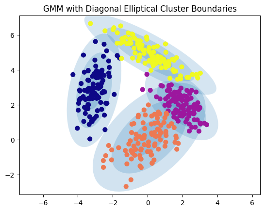
Points near the cluster boundaries have lower certainty, reflected in smaller marker sizes.
Flexible Cluster Shapes: GMM can model elliptical clusters, with diffent standard deviations, unlike k-Means, which assumes spherical clusters with uniform cluster sizes.
# Parameters for the blobs
n_samples = [400, 100, 100]
centers = [(0, 0), (4, 4), (-4, 4)]  # Center coordinates
cluster_std = [2., 0.5, 0.5]  # Standard deviations for each blob

# Generate blobs
X, y = make_blobs(n_samples=n_samples, centers=centers, cluster_std=cluster_std, random_state=1)

# Plot GMM with elliptical boundaries
gmm = GaussianMixture(n_components=3, covariance_type='full', random_state=42)
plot_gmm(gmm, X)
plt.show()
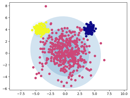
GMM is able to model more complex, elliptical cluster boundaries, addressing one of the main limitations of k-Means.
15.6. Expectation-Maximization (EM) Algorithm and Latent Variables#
The Expectation-Maximization (EM) algorithm is a widely-used technique in probabilistic models to estimate parameters in cases where some information is missing or hidden. These missing values are known as latent variables, unobserved factors that influence the data but are not directly visible. EM is powerful because it allows us to infer both the cluster membership of data points and, in more complex models, the internal structure of each cluster, such as its shape and spread.
For clustering tasks, latent variables can represent two main types of information:
Cluster Membership: This latent variable indicates which cluster each data point belongs to. In simpler models like k-means, cluster membership is treated as a discrete, “hard” assignment, meaning each data point is assigned entirely to one cluster. In more flexible models like Gaussian Mixture Models (GMMs), cluster membership is a “soft” assignment, where each data point has a probability of belonging to each cluster.
Cluster Structure: In GMMs and other probabilistic models, latent variables also describe the covariance structure within each cluster. This structure, captured by covariance matrices, allows each cluster to have its own unique shape and orientation, enabling the model to represent elliptical clusters or clusters with different spreads and dependencies between variables.
15.6.1. EM Algorithm and Cluster Membership#
In models like k-means, cluster membership is binary: each data point is assigned fully to one cluster. This approach can be understood within the EM framework by treating cluster membership as a discrete probability distribution with values of 0 or 1, indicating hard assignments.
For example:
k-Means can be considered a special case of the EM algorithm**, where each point is assigned entirely to the nearest cluster (E-Step), and then the cluster centroids are updated (M-Step) to minimize the total within-cluster variance.
In more sophisticated models like GMMs, cluster membership is “soft,” with each data point partially assigned to each cluster based on probability. This approach gives greater flexibility in representing clusters with overlapping regions and assigning partial membership to data points near cluster boundaries.
15.6.2. How the EM Algorithm Works#
The EM algorithm iteratively performs two key steps to refine both the cluster membership and the internal structure of each cluster:
Expectation (E) Step: In this step, based on the current estimates of the model parameters, we calculate the probability that each data point belongs to each cluster. This probability can be binary in k-means, where each point is assigned exclusively to one cluster, or continuous in GMMs, where each point is assigned a probability for each cluster. This step provides an estimate of the latent variables related to cluster membership.
Maximization (M) Step: Given the updated cluster memberships, we then re-estimate the model parameters to maximize the likelihood of observing the data. In k-means, this involves updating the cluster centroids. In GMMs, we not only update the mean of each cluster but also its covariance matrix, which captures the spread and orientation of each Gaussian component. This covariance matrix is essential in GMMs because it enables clusters to be elliptical and oriented in any direction, capturing richer relationships in the data.
15.6.3. Example: Gaussian Mixture Models and Covariance as Latent Structure#
Consider data that you suspect comes from a mixture of several Gaussian distributions, each with its own unique shape and spread. In this case, the latent variables include both:
Cluster Membership: The probability that each data point was generated by each Gaussian component, providing a “soft” assignment of data points to clusters.
Cluster Covariance: The covariance matrix of each Gaussian component, which describes the shape, size, and orientation of each cluster, allowing the model to capture dependencies and correlations among variables.
Using the EM algorithm in this setting, you would:
Start with initial guesses for the parameters of each Gaussian component, including its mean and covariance matrix.
E-Step: Compute the probability of each data point belonging to each Gaussian based on the current parameters. These probabilities act as “soft” assignments for cluster membership.
M-Step: Update the parameters for each Gaussian component, including the mean and covariance matrix, by maximizing the likelihood of observing the data with these updated assignments. The covariance matrix captures the internal structure, making it possible to model elliptical clusters and handle varying cluster sizes and orientations.
Through this iterative process, the EM algorithm provides estimates for both the cluster memberships and the structural parameters (mean and covariance), refining our understanding of the hidden cluster structure.
15.6.4. EM Algorithm’s Flexibility Beyond Clustering#
The EM algorithm’s iterative process of refining latent variables and model parameters is useful in many contexts beyond clustering:
In Hidden Markov Models (HMMs), the latent variables represent the hidden states that underlie observed sequences.
In factor analysis, latent variables might represent hidden factors that explain correlations among observed variables.
In topic modeling, latent variables capture hidden themes within documents, providing probabilistic assignments of words to topics.
Overall, the EM algorithm is a versatile approach that adapts to models of various complexities. By handling both discrete and continuous latent variables, EM enables us to model both simple cluster assignments, as in k-means, and richer, continuous structural relationships, as in GMMs. This ability to estimate hidden structures and dependencies makes EM a foundational tool in probabilistic modeling and unsupervised learning.
15.7. Comparison between k-Means and GMM#
The following table highlights the similarities and differences between the k-Means and GMM algorithms in terms of their iteration steps:
Step |
\(k\)-Means |
GMM |
|---|---|---|
Init |
Select \(K\) cluster centers \((\mathbf{m}_1^{(1)}, \ldots, \mathbf{m}_K^{(1)})\) |
\(K\) components with means \(\mu_k\), covariance \(\Sigma_k\), and mixing coefficients \(P_k\) |
E: |
Allocate data points to clusters: |
Update the probability that component \(k\) generated data point \(\mathbf{x}_n\): |
\[S_i^{(t)} = \{\mathbf{x}_p: ||\mathbf{x}_p - \mathbf{m}_i^{(t)}||^2 \le ||\mathbf{x}_p - \mathbf{m}_j^{(t)}||^2 \; \forall j \}\]
|
\[\gamma_{nk} = \frac{P_k \mathcal{N}(\mathbf{x}_n | \mu_k, \Sigma_k)}{\sum_{j=1}^K P_j \mathcal{N}(\mathbf{x}_n | \mu_j, \Sigma_j)} \]
|
|
M: |
Re-estimate cluster centers: |
Calculate estimated number of cluster members \(N_k\), means \(\mu_k\), covariance \(\Sigma_k\), and mixing coefficients \(P_k\): |
\[\mathbf{m}_i^{(t+1)} = \frac{1}{|S_i^{(t)}|} \sum_{\mathbf{x}_j \in S_i^{(t)}} \mathbf{x}_j \]
|
\[\begin{split}N_k = \sum_{n=1}^N \gamma_{nk}, \\
\mu_k^{\text{new}} = \frac{1}{N_k} \sum_{n=1}^N \gamma_{nk} \mathbf{x}_n, \\
\Sigma_k^{\text{new}} = \frac{1}{N_k} \sum_{n=1}^N \gamma_{nk} (\mathbf{x}_n - \mu_k^{\text{new}})(\mathbf{x}_n - \mu_k^{\text{new}})^T, \\
P_k^{\text{new}} = \frac{N_k}{N}\end{split}\]
|
|
Stop: |
Stop when there are no changes in cluster assignments. |
Stop when the log-likelihood does not increase |
\[\ln \Pr(\mathbf{x}|\boldsymbol{\mu}, \boldsymbol{\Sigma}, \mathbf{P}) = \sum_{n=1}^N \ln \left( \sum_{k=1}^K P_k \mathcal{N}(\mathbf{x}_n | \boldsymbol{\mu}_k, \boldsymbol{\Sigma}_k) \right)\]
|