7. Validation

7.1. The Importance of Independent Validation Sets in Machine Learning

In machine learning, the use of independent validation sets is crucial for evaluating model performance and avoiding one of the most common pitfalls: overfitting. Overfitting occurs when a model is trained to perform exceptionally well on the training data but fails to generalize to new, unseen data. This typically happens when the model is excessively complex for the given task or when it memorizes the noise and peculiarities of the training dataset instead of learning the underlying patterns.

An independent validation set helps to detect overfitting by providing a dataset that is separate from the training set, allowing for an unbiased evaluation of the model’s performance. Moreover, selecting the model that performs best on an independent validation set ensures that we are choosing a model that is most likely to generalize well to new data, rather than simply performing well on the training data.

To split data into training and validation sets, scikit-learn provides a convenient method called train_test_split. This function allows us to easily partition the data into training and test sets, ensuring that we have separate data to evaluate the model before proceeding with more advanced validation techniques. By default, train_test_split uses 75% of the data for training and 25% for testing, but this can be adjusted using the test_size parameter.

7.1.1. Example of Overfitting

Below, we create a small dataset of 10 data points, and we compare the performance of two polynomial regression models—a simple linear model and an overfitted higher-order polynomial model.

import numpy as np
import matplotlib.pyplot as plt
from sklearn.preprocessing import PolynomialFeatures
from sklearn.linear_model import LinearRegression
from sklearn.metrics import mean_squared_error
from sklearn.model_selection import train_test_split

# Generating synthetic data
np.random.seed(42)
x = np.linspace(-3, 3, 10).reshape(-1, 1)
y = 0.5 * x**2 + np.random.normal(0, 0.5, x.shape)

# Splitting the data into training and test sets
x_train, x_val, y_train, y_val = train_test_split(x, y, test_size=0.3, random_state=42)

# Creating a linear regression model and a higher-order polynomial regression model
linear_model = LinearRegression()
quad_model = LinearRegression()
poly_model = LinearRegression()
quadratic_features = PolynomialFeatures(degree=2)
polynomial_features = PolynomialFeatures(degree=8)

# Fitting the models
linear_model.fit(x_train, y_train)
x_quad = quadratic_features.fit_transform(x_train)
quad_model.fit(x_quad, y_train)
x_poly = polynomial_features.fit_transform(x_train)
poly_model.fit(x_poly, y_train)

# Predicting using the fitted models
y_linear_train_pred = linear_model.predict(x_train)
y_linear_val_pred = linear_model.predict(x_val)
y_quad_train_pred = quad_model.predict(quadratic_features.transform(x_train))
y_quad_val_pred = quad_model.predict(quadratic_features.transform(x_val))
y_poly_train_pred = poly_model.predict(polynomial_features.transform(x_train))
y_poly_val_pred = poly_model.predict(polynomial_features.transform(x_val))

# Calculating and printing train and validation errors for each model
linear_train_error = mean_squared_error(y_train, y_linear_train_pred)
linear_val_error = mean_squared_error(y_val, y_linear_val_pred)
quad_train_error = mean_squared_error(y_train, y_quad_train_pred)
quad_val_error = mean_squared_error(y_val, y_quad_val_pred)
poly_train_error = mean_squared_error(y_train, y_poly_train_pred)
poly_val_error = mean_squared_error(y_val, y_poly_val_pred)

print(f"Linear Model - Train Error: {linear_train_error:.2f}, Validation Error: {linear_val_error:.2f}")
print(f"Quadratic Model - Train Error: {quad_train_error:.2f}, Validation Error: {quad_val_error:.2f}")
print(f"High-Degree Model - Train Error: {poly_train_error:.2f}, Validation Error: {poly_val_error:.2f}")

# Plotting the data
x_test = np.linspace(-3, 3, 100).reshape(-1, 1)
y_linear_pred = linear_model.predict(x_test)
y_quad_pred = quad_model.predict(quadratic_features.transform(x_test))
y_poly_pred = poly_model.predict(polynomial_features.transform(x_test))

plt.scatter(x_train, y_train, color='black', label='Training Data')
plt.scatter(x_val, y_val, color='gray', label='Validation Data')
plt.plot(x_test, y_linear_pred, label='Linear Model (Underfitting)', color='blue')
plt.plot(x_test, y_quad_pred, label='Quadratic Model', color='green')
plt.plot(x_test, y_poly_pred, label='High-Degree Model (Overfitting)', color='red')
plt.legend()
plt.xlabel("x")
plt.ylabel("y")
plt.show()

Linear Model - Train Error: 2.90, Validation Error: 1.85
Quadratic Model - Train Error: 0.08, Validation Error: 0.28
High-Degree Model - Train Error: 0.00, Validation Error: 67.64

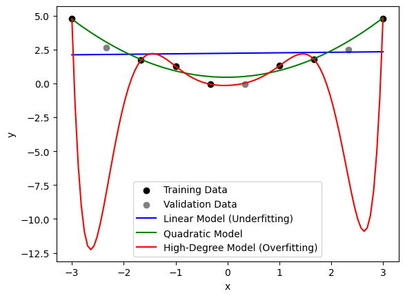
In the above code, we create a simple quadratic dataset, and fit both a linear regression model, a second-degree polynomial model, and an eighth-degree polynomial model. We also split the dataset into training and validation sets using train_test_split. The linear model appears to miss an important trend in the data and is hence underfitting. The eighth-degree model fits the training data almost perfectly, capturing all of the data points and the noise, but it is unlikely to perform well on new data—an example of overfitting.

7.1.2. Cross Validation to the Rescue

A problem with reserving data for a separate validation set is that we have to reserve precious data for either training or testing. Idealy, one would like to train and test on as much data as possible. Therefore, to evaluate how well a model will perform on new, unseen data, it’s important to use validation techniques such as cross validation. Cross validation is a strategy that partitions the available data into multiple subsets, or folds, allowing the model to be trained on one subset and validated on another. This ensures that each data point is eventually used both for training and validation. The method allows us to assess how well a model generalizes to unseen data, providing an estimate of the expected accuracy on new samples – still using all available data.

In k-fold cross validation, the dataset is split into k equally sized folds. The model is trained k times, each time using a different fold as the validation set and the remaining folds for training. The average of the validation metrics across all folds gives a more robust estimate of the model’s performance compared to using a single validation set.

7.1.3. Illustration of Three-Fold Cross Validation

Imagine we have a dataset with six data points, represented as A, B, C, D, E, F. In three-fold cross validation, we can split this dataset into three subsets, each containing two data points. For example:

• Fold 1: Training on [C, D, E, F], Validation on [A, B]

• Fold 2: Training on [A, B, E, F], Validation on [C, D]

• Fold 3: Training on [A, B, C, D], Validation on [E, F]

Each fold is used for validation once, and the model is trained on the remaining data. This way, every data point contributes to both training and evaluation, reducing the risk of overfitting and improving the robustness of the performance estimate.

Here is a code example illustrating three-fold cross validation with six data points:

from sklearn.model_selection import KFold

# Example dataset with six data points
x_example = np.array([[1], [2], [3], [4], [5], [6]])
y_example = np.array([1, 4, 9, 16, 25, 36])

# Setting up three-fold cross validation
kf_example = KFold(n_splits=3, shuffle=True, random_state=42)

for fold, (train_index, test_index) in enumerate(kf_example.split(x_example)):
    print(f"Fold {fold + 1}: Training on {x_example[train_index].flatten()}, Validation on {x_example[test_index].flatten()}")

Fold 1: Training on [3 4 5 6], Validation on [1 2]
Fold 2: Training on [1 2 4 5], Validation on [3 6]
Fold 3: Training on [1 2 3 6], Validation on [4 5]

This code demonstrates how the dataset is split into three folds, with each fold being used for validation once while the remaining data points are used for training. This helps ensure that all data points are used for both training and validation, providing a comprehensive evaluation of the model’s performance.

        flowchart TB
    subgraph Dataset [Dataset]
      A["    Fold 1    "]
      B["    Fold 2    "]
      C["    Fold 3    "]
    end

    subgraph Mod1 [Model 1]
        T1[Train Model] --> M1[[Model 1]]
        M1 --> V1[Validate Model on unseen data]
    end
    subgraph Mod2 [Model 2]
        T2[Train Model] --> M2[[Model 2]]
        M2 --> V2[Validate Model on unseen data]
    end
    subgraph Mod3 [Model 3]
        T3[Train Model] --> M3[[Model 3]]
        M3 --> V3[Validate Model on unseen data]
    end

    %% Fold 1
    A --> T1
    B --> T1
    C -. Test .-> V1

    %% Fold 2
    A --> T2
    B -. Test .-> V2
    C --> T2

    %% Fold 3
    A -. Test .-> V3
    B --> T3
    C --> T3
    

7.1.4. Cross Validation to detect overfitting

In the following code, we demonstrate how to use scikit-learn’s KFold cross validation with three-fold cross validation for a simple linear regression model:

from sklearn.model_selection import KFold
from sklearn.pipeline import make_pipeline

# Creating a pipeline for polynomial regression with degree 2 and 8
pipeline_2 = make_pipeline(PolynomialFeatures(degree=2), LinearRegression())
pipeline_8 = make_pipeline(PolynomialFeatures(degree=8), LinearRegression())

# Setting up three-fold cross validation
kf = KFold(n_splits=3, shuffle=True, random_state=42)
scores_2, scores_8 = [], []

for train_index, test_index in kf.split(x):
    x_train, x_test = x[train_index], x[test_index]
    y_train, y_test = y[train_index], y[test_index]
    # Fit and test second degree polynomia
    pipeline_2.fit(x_train, y_train)
    y_pred = pipeline_2.predict(x_test)
    mse = mean_squared_error(y_test, y_pred)
    scores_2.append(mse)
    # Fit and test eith degree polynomia
    pipeline_8.fit(x_train, y_train)
    y_pred = pipeline_8.predict(x_test)
    mse = mean_squared_error(y_test, y_pred)
    scores_8.append(mse)

# Calculating and printing the mean score
print(f"Mean cross-validated MSE, for 2nd degree: {np.mean(scores_2):.2f} and for 8th degree: {np.mean(scores_8):.2f}")

Mean cross-validated MSE, for 2nd degree: 0.23 and for 8th degree: 11003.98

In this code, we use KFold to split the dataset into three folds. The for loop iterates through each fold, training the model on the training set and evaluating it on the test set. The mean squared error (MSE) is calculated for each fold and averaged to give a more robust measure of model performance. By splitting the data into different training and validation sets multiple times, cross validation helps to detect overfitting and provides a more reliable measure of model generalizability.

7.2. Hyperparameter Selection

Hyperparameters are parameters of the machine learning model that are not learned from the training data but are instead set before training begins. Examples include the number of trees in a random forest, the learning rate in gradient descent, or the degree of regularization. Proper selection of hyperparameters is crucial to maximize a model’s performance, and two common methods for finding the best combination of hyperparameters are grid search and nested cross validation.

7.2.1. Grid Search for Hyperparameter Tuning

Grid search is a brute-force method for finding the optimal hyperparameter values for a given model. It involves specifying a grid of hyperparameter values and then training and evaluating the model for each combination of parameters. The combination that yields the best performance on the validation set is selected as the final set of hyperparameters.

Let’s consider an example where we are training a Lasso regression model, and we want to determine the optimal value for the hyperparameter, \(\alpha\). Lasso regression is a linear model that includes L1 regularization, which helps to prevent overfitting by adding a penalty to the magnitude of the coefficients, effectively setting some of them to zero. With grid search, we define a range of possible values for \(\alpha\) and iterate over each value, training and evaluating the model at each step.

The following code demonstrates the use of GridSearchCV in scikit-learn to perform a grid search over the regularization parameter of a Lasso regression model:

import numpy as np
from sklearn.model_selection import GridSearchCV
from sklearn.linear_model import Lasso
from sklearn.preprocessing import PolynomialFeatures
from sklearn.pipeline import make_pipeline
from sklearn.preprocessing import StandardScaler

# Generating synthetic data from a second order polynomial with Gaussian noise
np.random.seed(42)
x = np.linspace(-3, 3, 100).reshape(-1, 1)
y = 0.5 * x**2 + np.random.normal(0, 0.5, x.shape)

# Creating a pipeline for polynomial regression with Lasso regularization
model = make_pipeline(PolynomialFeatures(degree=5), StandardScaler(), Lasso(max_iter=10000))

# Defining the parameter grid
param_grid = {'lasso__alpha': [0.01, 0.1, 1, 10, 100]}

# Setting up GridSearchCV
grid_search = GridSearchCV(model, param_grid, cv=3, scoring='neg_mean_squared_error')

# Performing the grid search
grid_search.fit(x, y)

# Printing the best parameters
print(f"Best hyperparameters: {grid_search.best_params_}")

# Printing the coefficients for each value of alpha
for i, estimator in enumerate(grid_search.cv_results_['params']):
    alpha = estimator['lasso__alpha']
    model.set_params(**estimator)
    model.fit(x, y)
    lasso = model.named_steps['lasso']
    print(f"Alpha: {alpha}, Coefficients for model {i + 1}: {lasso.coef_}")

Best hyperparameters: {'lasso__alpha': 0.1}
Alpha: 0.01, Coefficients for model 1: [ 0.          0.10553842  1.23103587 -0.          0.1622308  -0.11625395]
Alpha: 0.1, Coefficients for model 2: [ 0.          0.          1.18498276 -0.          0.11636712 -0.        ]
Alpha: 1, Coefficients for model 3: [ 0.          0.          0.39640516 -0.          0.         -0.        ]
Alpha: 10, Coefficients for model 4: [ 0.  0.  0. -0.  0. -0.]
Alpha: 100, Coefficients for model 5: [ 0.  0.  0. -0.  0. -0.]

In the code above, we generate synthetic data from a second-order polynomial with Gaussian noise. We specify a grid of values for the regularization parameter \(\alpha\). The GridSearchCV function performs cross validation for each value of \(\alpha\) and returns the value that yields the best performance. Note that we set the parameter cv=3 to perform three-fold cross validation, which helps to reduce bias and variance in the results.

7.2.2. Nested Cross Validation

One limitation of the standard grid search approach is that it is prone to overfitting if the same validation set is used to both tune hyperparameters and evaluate model performance. To address this issue, nested cross validation is used.

In nested cross validation, there are two loops:

• The outer loop is used to split the data into training and testing sets, ensuring that the test set remains completely independent.

• The inner loop is used to perform grid search on the training set, determining the best hyperparameters.

The model is trained and validated using the inner loop, and its final performance is evaluated using the held-out data from the outer loop. This process is repeated multiple times, each time using different splits of the data, to ensure robustness and minimize the risk of overfitting.

The following code demonstrates how nested cross validation can be performed using scikit-learn:

from sklearn.model_selection import cross_val_score
from sklearn.model_selection import KFold

# Setting up the inner and outer cross validation loops
inner_cv = KFold(n_splits=3, shuffle=True, random_state=42)
outer_cv = KFold(n_splits=5, shuffle=True, random_state=42)

# Using GridSearchCV within cross_val_score for nested cross validation
grid_search = GridSearchCV(model, param_grid, cv=inner_cv, scoring='neg_mean_squared_error')
nested_scores = cross_val_score(grid_search, x, y, cv=outer_cv)

print(f"Nested cross-validated MSE: {-nested_scores.mean():.2f} (+/- {nested_scores.std():.2f})")

Nested cross-validated MSE: 0.21 (+/- 0.10)

In this code, the outer loop (outer_cv) splits the dataset into 5 folds. For each split, the inner loop (inner_cv) uses 3-fold cross validation to perform a grid search over the hyperparameters. This ensures that hyperparameters are optimized on an independent portion of the data, leading to a more accurate and unbiased estimate of model performance. As you see from above, a feature of the cross validation is that it provides posibility to calculate variance estimates of performance figures, since you have calculated the error over a number of predictors for number of validation sets.