23. Appendix: Some Maths

23.1. Linear algebra

23.1.1. Row Vector

A row vector is a 1-dimensional array consisting of a single row of elements. For example, a row vector with three elements can be written as:

\[ \mathbf{r} = [r_1, r_2, r_3] \]

23.1.2. Column Vector

A column vector is a 1-dimensional array consisting of a single column of elements. It can be thought of as a matrix with one column. For instance, a column vector with three elements appears as:

\[\begin{split} \mathbf{c} = \begin{bmatrix} c_1 \\ c_2 \\ c_3 \end{bmatrix} \end{split}\]

23.1.3. Matrix

A matrix is a rectangular array of numbers arranged in rows and columns. For example, a matrix with two rows and three columns is shown as:

\[\begin{split} \mathbf{A} = \begin{bmatrix} a_{11} & a_{12} & a_{13} \\ a_{21} & a_{22} & a_{23} \end{bmatrix} \end{split}\]

23.1.4. Transpose Operator

The transpose of a matrix is obtained by swapping its rows with its columns. The transpose of matrix \(\mathbf{A}\) is denoted \(\mathbf{A}^T\). For the given matrix \(\mathbf{A}\), the transpose is:

\[\begin{split} \mathbf{A}^T = \begin{bmatrix} a_{11} & a_{21} \\ a_{12} & a_{22} \\ a_{13} & a_{23} \end{bmatrix} \end{split}\]

23.1.5. Multiplication between Vectors

Vector multiplication can result in either a scalar or a matrix:

• Dot product: Multiplication of the transpose of a column vector \(\mathbf{a}\) with another column vector \(\mathbf{b}\) results in a scalar. This is also known as the inner product:

\[ \mathbf{a}^T \mathbf{b} = a_1b_1 + a_2b_2 + a_3b_3 \]

• Outer product: The multiplication of a column vector \(\mathbf{a}\) by the transpose of another column vector \(\mathbf{b}\) results in a matrix:

\[\begin{split} \mathbf{a} \mathbf{b}^T = \begin{bmatrix} a_1b_1 & a_1b_2 & a_1b_3 \\ a_2b_1 & a_2b_2 & a_2b_3 \\ a_3b_1 & a_3b_2 & a_3b_3 \end{bmatrix} \end{split}\]

23.1.6. Matrix Multiplication

The product of two matrices \(\mathbf{A}\) and \(\mathbf{B}\) is a third matrix \(\mathbf{C}\). Each element \(c_{ij}\) of \(\mathbf{C}\) is computed as the dot product of the \(i\)-th row of \(\mathbf{A}\) and the \(j\)-th column of \(\mathbf{B}\):

\[ c_{ij} = \sum_{k} a_{ik} b_{kj} \]

23.1.7. L2-norm (Euclidean norm)

The L2-norm of a vector \(\mathbf{x} = [x_1,\dots,x_n]^T\) (also called the Euclidean norm) measures its length and is defined as:

\[ \|\mathbf{x}\|_2 = \sqrt{\sum_{i=1}^n x_i^2}. \]

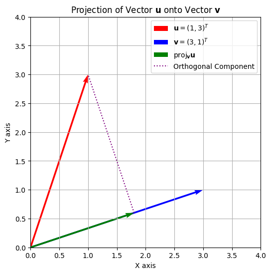
23.1.8. Projection

The projection of vector \(\mathbf{u}\) onto vector \(\mathbf{v}\) is given by:

\[ \text{proj}_{\mathbf{v}} \mathbf{u} = \frac{\mathbf{u}^T\mathbf{v}}{\mathbf{v}^T\mathbf{v}} \mathbf{v} \]

This represents the orthogonal projection of \(\mathbf{u}\) in the direction of \(\mathbf{v}\).

Show code cell source

Hide code cell source

import numpy as np
import matplotlib.pyplot as plt

u = np.array([1, 3])
v = np.array([3, 1])

# Recalculate the projection of u onto the new v
proj_u_on_v = np.dot(u, v) / np.dot(v, v) * v
orthogonal_component = u - proj_u_on_v

# Update plot with new vector v and its projection
plt.figure(figsize=(6, 6))
plt.quiver(0, 0, u[0], u[1], angles='xy', scale_units='xy', scale=1, color='r', label=r'$\mathbf{u}=(1,3)^T$')
plt.quiver(0, 0, v[0], v[1], angles='xy', scale_units='xy', scale=1, color='b', label=r'$\mathbf{v}=(3,1)^T$')
plt.quiver(0, 0, proj_u_on_v[0], proj_u_on_v[1], angles='xy', scale_units='xy', scale=1, color='g', label='proj$_{\mathbf{v}} \mathbf{u}$')

# Plot orthogonal line as a dotted line segment
end_point = proj_u_on_v + orthogonal_component
plt.plot([proj_u_on_v[0], end_point[0]], [proj_u_on_v[1], end_point[1]], 'purple', linestyle='dotted', label='Orthogonal Component')

# Set plot limits and aspect
plt.xlim(0, 4)
plt.ylim(0, 4)
plt.gca().set_aspect('equal', adjustable='box')

# Add a grid, legend, and labels
plt.grid(True)
plt.legend()
plt.title('Projection of Vector $\mathbf{u}$ onto Vector $\mathbf{v}$')
plt.xlabel('X axis')
plt.ylabel('Y axis')
plt.show()

23.1.9. Eigenvalue and Eigenvector

An eigenvalue \(\lambda\) and its corresponding eigenvector \(\mathbf{v}\) of a matrix \(\mathbf{A}\) satisfy the equation:

\[ \mathbf{A} \mathbf{v} = \lambda \mathbf{v} \]

23.1.10. Gradient

The gradient of a multivariable function \(f(\mathbf{x})\) is a vector of partial derivatives, which points in the direction of the steepest ascent of \(f\):

\[\begin{split} \nabla f(\mathbf{x}) = \begin{bmatrix} \frac{\partial f}{\partial x_1} \\ \frac{\partial f}{\partial x_2} \\ \vdots \\ \frac{\partial f}{\partial x_n} \end{bmatrix} \end{split}\]

23.2. Basics of Probability

23.2.1. Descriptive Statistics

23.2.1.1. Mean

The mean or expected value of a set of numbers is the average of all the values. For a set \( X = \{x_1, x_2, \dots, x_n\} \), the mean \( \mu \) is calculated as:

\[ \mu = \frac{1}{n} \sum_{i=1}^n x_i \]

23.2.1.2. Variance

The variance measures the spread of a set of numbers from their mean. For a sample set \( X \), the variance \( \sigma^2 \) using the maximum likelihood estimate is defined as:

\[ \sigma^2 = \frac{1}{n-1} \sum_{i=1}^n (x_i - \mu)^2 \]

23.2.1.3. Covariance

Covariance is a measure of how much two random variables change together. For variables \( X \) and \( Y \), the covariance using the maximum likelihood estimate is defined as:

\[ \text{cov}(X, Y) = \frac{1}{n-1} \sum_{i=1}^n (x_i - \mu_X)(y_i - \mu_Y) \]

23.2.1.4. Probability Distributions

23.2.1.4.1. Uniform Distribution

The uniform distribution is a probability distribution where every outcome is equally likely over a given interval \([a, b]\). Its probability density function (pdf) is:

\[ f(x) = \frac{1}{b-a} \quad \text{for } x \in [a, b] \]

23.2.1.5. Normal Distribution

The normal distribution is a probability distribution that is symmetric about the mean, showing that data near the mean are more frequent in occurrence than data far from the mean. Its pdf is given by:

\[ f(x) = \frac{1}{\sigma\sqrt{2\pi}} e^{-\frac{(x - \mu)^2}{2\sigma^2}} \]

23.2.1.6. Probability Density Function (PDF)

The probability density function (pdf) of a continuous random variable is a function that describes the likelihood of the random variable taking on a specific value. The area under the pdf curve between two values represents the probability of the variable falling within that range.

23.2.1.7. Cumulative Distribution Function (CDF)

The cumulative distribution function (cdf) of a random variable \( X \) gives the probability that \( X \) will take a value less than or equal to \( x \). It is defined as:

\[ F(x) = P(X \leq x) \]

23.2.1.8. Expectation Value

The expectation value of a random variable is the long-run average value of repetitions of the experiment it represents. For a random variable \( X \) with a probability function \( p(x) \), the expectation is given by:

\[ E[X] = \sum_{x} x \cdot p(x) \quad \text{(discrete)} \quad \text{or} \quad E[X] = \int_{-\infty}^{\infty} x \cdot f(x) dx \quad \text{(continuous)} \]

23.2.2. Probabilistic Inference

23.2.2.1. Likelihood

The likelihood function expresses how well different parameter values explain the observed data. For continuous data, it is written as \(L(\theta \mid x) = p(x \mid \theta),\) and for discrete data as \(L(\theta \mid x) = \Pr(x \mid \theta).\)

Although the likelihood has the same mathematical form as a probability or density function, its interpretation differs: in the likelihood, the data (\(x\)) are fixed and (\(\theta\)) varies. The likelihood is not a probability distribution over (\(\theta\)); its role is to compare parameter values in light of the data.

23.2.2.2. Maximum Likelihood

The maximum likelihood estimate (MLE) is the parameter value that maximizes the likelihood function:

\[ \hat{\theta}^*_{\text{MLE}} = \arg\max_{\theta} L(\theta \mid x). \]

It identifies the parameter that makes the observed data most probable (or most dense) under the model. MLEs are widely used because, under general conditions, they are consistent, efficient, and asymptotically normal. In practice, the likelihood is often maximized numerically using gradient-based or expectation–maximization algorithms.

23.2.2.3. Prior Probability

The prior probability (\(\Pr(\theta)\)) (or density (\(p(\theta)\))) represents our beliefs about parameter values before any data are observed. Priors can encode earlier experimental knowledge, theoretical limits, or subjective expectations. When little information is available, weakly informative or noninformative priors are used to prevent the prior from dominating the inference. In continuous models, the prior is a density (\(p(\theta)\)) satisfying (\(\int p(\theta),d\theta = 1\)); in discrete models, it is a probability mass function (\(\Pr(\theta)\)) summing to one.

23.2.2.4. Posterior Probability

After observing data (x), the prior is updated using Bayes’ theorem:

\[ p(\theta \mid x) = \frac{p(x \mid \theta),p(\theta)}{p(x)} \quad \text{or} \quad \Pr(\theta \mid x) = \frac{\Pr(x \mid \theta),\Pr(\theta)}{\Pr(x)}. \]

The resulting posterior distribution combines prior information with the information from the data through the likelihood. The denominator,

\[ p(x) = \int p(x \mid \theta),p(\theta),d\theta, \]

(or the corresponding sum for discrete variables) is the marginal likelihood or evidence, ensuring that the posterior integrates or sums to one. The posterior forms the basis for Bayesian inference, from which we can compute summaries such as the posterior mean, variance, or mode.

23.2.3. Relationships Between Random Variables

23.2.3.1. Joint Probability Distributions

A joint probability distribution describes the probability (or density) of two or more random variables taking specific values together. For two variables (\(X\)) and (\(Y\)),

\[ \Pr(X = x, Y = y) \quad \text{or} \quad p(x, y) \]

denotes their joint distribution. From it, we can obtain:

\[ \Pr(X = x) = \sum_y \Pr(X = x, Y = y), \quad p(x) = \int p(x, y),dy, \]

and conditional relationships such as

\[ \Pr(Y = y \mid X = x) = \frac{\Pr(X = x, Y = y)}{\Pr(X = x)}, \quad p(y \mid x) = \frac{p(x, y)}{p(x)}. \]

23.2.3.2. Marginal Probability Distributions

A marginal probability distribution gives the probability or density of a subset of variables, obtained by summing or integrating out the others from a joint distribution. For example, from a joint distribution of (\(X\)) and (\(Y\)):

\[ \Pr(X = x) = \sum_y \Pr(X = x, Y = y), \quad p(x) = \int p(x, y),dy. \]

This process is called marginalization. The resulting marginal describes the distribution of (\(X\)) alone, regardless of (\(Y\)). Marginals are useful for computing expected values, normalizing posteriors, and analyzing subsystems within larger probabilistic models. In Bayesian inference, the marginal distribution of the data,

\[ p(x) = \int p(x \mid \theta),p(\theta),d\theta, \]

plays a key role as the normalizing constant in Bayes’ theorem and is sometimes referred to as the evidence.