16. Cluster analysis of TCGA breast cancer sets#
Here we are perfoming a k-means analysis of two different datasets within the TCGA.
First we retrieve the breast cancer RNAseq data as well as the clinical classification of the sets from cbioportal.org. The code for the retrieval of this data set is not important for the understanding of the analysis, but the code is kept for completness. Execute the code and proceed to next step.
import pandas as pd
import seaborn as sns
import numpy as np
import sys
IN_COLAB = 'google.colab' in sys.modules
if IN_COLAB:
    ![ ! -f "dsbook/README.md" ] && git clone https://github.com/statisticalbiotechnology/dsbook.git
    my_path = "dsbook/dsbook/common/"
else:
    my_path = "../common/"
sys.path.append(my_path) # Read local modules for tcga access and qvalue calculations
import load_tcga as tcga

brca = tcga.get_expression_data(my_path + "../data/brca_tcga_pub2015.tar.gz", 'https://cbioportal-datahub.s3.amazonaws.com/brca_tcga_pub2015.tar.gz',"data_mrna_seq_v2_rsem.txt")
brca_clin = tcga.get_clinical_data(my_path + "../data/brca_tcga_pub2015.tar.gz", 'https://cbioportal-datahub.s3.amazonaws.com/brca_tcga_pub2015.tar.gz',"data_clinical_sample.txt")
File extracted to ../data/brca_tcga_pub2015
File extracted to ../data/brca_tcga_pub2015
Before any further analysis we clean our data. This includes removal of genes where no transcripts were found for any of the samples , i.e. their values are either NaN or zero.
The data is also log transformed. It is generally assumed that expression values follow a log-normal distribution, and hence the log transformation implies that the new values follow a nomal distribution.
brca.dropna(axis=0, how='any', inplace=True)
brca = brca.loc[~(brca<=0.0).any(axis=1)]
brca = pd.DataFrame(data=np.log2(brca),index=brca.index,columns=brca.columns)
16.1. Clustering with k-means#
We first try to separate our data, just as it stands, into two clusters. This is done with k-means clustering with k=2.
from sklearn.cluster import KMeans
import numpy as np

X = brca.values.T
kmeans = KMeans(n_clusters=2, random_state=0).fit(X)
label_df = pd.DataFrame(columns=brca.columns,index=["kmeans_2"],data=[list(kmeans.labels_)])
brca_clin=pd.concat([brca_clin,label_df])
We investigate the clusters to see what size they have.
label_df.loc["kmeans_2"].value_counts()
kmeans_2
0    632
1    185
Name: count, dtype: int64
Do we see any reason for the clustering’s divide of the data? There is actually one appealing interpretation.
We can compare the clusters to wich patients that have been marked as Progesterone receptor Negative and Estrogen receptor Negative, i.e. the patologist did not fin that those receptors were expressed by the tumor. Such cancers are known to behave different than other cancers, and are less amendable to hormonal theraphy.
brca_clin.loc["2N"]= (brca_clin.loc["PR_STATUS_BY_IHC"]=="Negative") & (brca_clin.loc["ER_STATUS_BY_IHC"]=="Negative")
confusion_matrix = pd.crosstab(brca_clin.loc['2N'], brca_clin.loc['kmeans_2'], rownames=['PR-&ER-'], colnames=['Cluster'])
confusion_matrix
| Cluster | 0 | 1 |
|---|---|---|
| PR-&ER- | ||
| False | 611 | 44 |
| True | 21 | 141 |
So this time the cluster seem to reflect the different nature of the samples. Cluster 1 contains the bulk of all patients that are both ER- and PR-.
16.2. Gausian Mixturte models#
Another method to cluster data is Gausian Mixture Models (GMM). GMMs have a number of different applicats, however, here we use them for clustering. A key difference to k-Means, is that GMMs form their components (clusters) with different sense of distance in different feature directions directions. Below we perform a GMM clustering for two separate components.
from sklearn.mixture import GaussianMixture,BayesianGaussianMixture
gmm = GaussianMixture(n_components=2, covariance_type='diag', random_state=0).fit(X)
label_df = pd.DataFrame(columns=brca.columns,index=["GMM_2"],data=[list(gmm.predict(X))])
brca_clin=pd.concat([brca_clin,label_df])
Again we compare our components to the explanation that the two clusters manage to capture the difference between tumors that are both ER- and PR- and other tumors.
confusion_matrix = pd.crosstab(brca_clin.loc['2N'], brca_clin.loc['GMM_2'], rownames=['PR-&ER-'], colnames=['Component'])
confusion_matrix
| Component | 0 | 1 |
|---|---|---|
| PR-&ER- | ||
| False | 417 | 238 |
| True | 11 | 151 |
The GMMs seem to have less clear separation between the two cases, with a fair number of the non ER-&PR- patients being included in cluster 0.
16.2.1. Bayesian Gausian Mixture Models#
A nice way to impement GMMs is in a Bayesian framework. An advantage of such models is the possibility not have to specify the number of components k, but instead let the algorithm select it for you, given an upper bound of k. The following exampe, taken from the scikit-learn documentation makes a direct demonstration of why that is useful on a two dimensional feature space.
import itertools
from scipy import linalg
import matplotlib.pyplot as plt
import matplotlib as mpl

color_iter = itertools.cycle(['navy', 'c', 'cornflowerblue', 'gold',
                              'darkorange'])


def plot_results(X_, Y_, means, covariances, index, title):
    splot = plt.subplot(2, 1, 1 + index)
    for i, (mean, covar, color) in enumerate(zip(
            means, covariances, color_iter)):
        v, w = linalg.eigh(covar)
        v = 2. * np.sqrt(2.) * np.sqrt(v)
        u = w[0] / linalg.norm(w[0])
        # as the DP will not use every component it has access to
        # unless it needs it, we shouldn't plot the redundant
        # components.
        if not np.any(Y_ == i):
            continue
        plt.scatter(X_[Y_ == i, 0], X_[Y_ == i, 1], .8, color=color)

        # Plot an ellipse to show the Gaussian component
        angle = np.arctan(u[1] / u[0])
        angle = 180. * angle / np.pi  # convert to degrees
        ell = mpl.patches.Ellipse(mean, v[0], v[1], angle=180.0 + angle, color=color)
        ell.set_clip_box(splot.bbox)
        ell.set_alpha(0.5)
        splot.add_artist(ell)

    plt.xlim(-9., 5.)
    plt.ylim(-3., 6.)
    plt.xticks(())
    plt.yticks(())
    plt.title(title)


# Number of samples per component
n_samples = 500

# Generate random sample, two components
np.random.seed(0)
C = np.array([[0., -0.1], [1.7, .4]])
X_ = np.r_[np.dot(np.random.randn(n_samples, 2), C),
          .7 * np.random.randn(n_samples, 2) + np.array([-6, 3])]

# Fit a Gaussian mixture with EM using five components
gmm = GaussianMixture(n_components=5, covariance_type='full').fit(X_)
plot_results(X_, gmm.predict(X_), gmm.means_, gmm.covariances_, 0,
             'Gaussian Mixture')

# Fit a Dirichlet process Gaussian mixture using five components
dpgmm = BayesianGaussianMixture(n_components=5,
                                        covariance_type='full').fit(X_)
plot_results(X_, dpgmm.predict(X_), dpgmm.means_, dpgmm.covariances_, 1,
             'Bayesian Gaussian Mixture\n(with a Dirichlet process prior)')
/opt/hostedtoolcache/Python/3.11.14/x64/lib/python3.11/site-packages/sklearn/mixture/_base.py:293: ConvergenceWarning: Best performing initialization did not converge. Try different init parameters, or increase max_iter, tol, or check for degenerate data.
  warnings.warn(
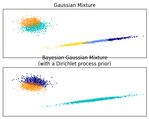
The GMM to the left tries to apply five different component to the data that seem to origin from two sources. The Bayesian implementation correctly recognizes that there are just two components, and sucessfully captures their spread.
We use the same technique, however instead of clustering our 20,000 dimensional data, we select a subset of 15 known cancer associated genes.
brca_names = ["ESR1", "SLC44A4", "SCUBE2", "FOXA1", "CA12", "NAT1", "BCAS1", "AFF3", "DNALI1", "CDCA7", "FOXC1", "SFRP1", "S100A9", "EN1", "PSAT1"]
Xlim = brca.loc[brca_names].values.T
bgmm = BayesianGaussianMixture(n_components=30, covariance_type='diag', random_state=1,max_iter=1000,n_init=10, tol=0.01).fit(Xlim)
label_df = pd.DataFrame(columns=brca.columns,index=["LimBGMM_30"],data=[list(bgmm.predict(Xlim))])
brca_clin=pd.concat([brca_clin,label_df])
label_df.loc["LimBGMM_30"].value_counts()
LimBGMM_30
6     226
19    135
26    125
11    119
18    116
20     68
3      21
15      4
25      2
17      1
Name: count, dtype: int64
The algoritm clusters the data into 10 different clusters, where the bulk of the samples are in the 5 largest clusters. The interpretation of this clustering is left to you as a reader.