18. PCA analysis of two lung cancer sets

Here we are perfoming a PCA of two different datasets within the TCGA. We will first merge the two datasets and subsequently try to separate the samples based on their principal components.

First we retrieve our two TCGA lungcancer data from cbioportal.org. One of the sets are from Lung Adenocarcinomas and the other is from Lung Squamous Cell Carcinomas. The code for the retrieval of this data set is not important for the understanding of the analysis, but can be found in the module tcga_read. Execute the code and proceed to next step.

import pandas as pd
import seaborn as sns
import numpy as np
import sys
IN_COLAB = 'google.colab' in sys.modules
if IN_COLAB:
    ![ ! -f "dsbook/README.md" ] && git clone https://github.com/statisticalbiotechnology/dsbook.git
    my_path = "dsbook/dsbook/common/"
else:
    my_path = "../common/"
sys.path.append(my_path) # Read local modules for tcga access and qvalue calculations
import load_tcga as tcga

luad = tcga.get_expression_data(my_path + "../data/luad_tcga_pan_can_atlas_2018.tar.gz", 'https://cbioportal-datahub.s3.amazonaws.com/luad_tcga_pan_can_atlas_2018.tar.gz',"data_mrna_seq_v2_rsem.txt")
lusc = tcga.get_expression_data(my_path + "../data/lusc_tcga_pan_can_atlas_2018.tar.gz", 'https://cbioportal-datahub.s3.amazonaws.com/lusc_tcga_pan_can_atlas_2018.tar.gz',"data_mrna_seq_v2_rsem.txt")

Downloading ../common/../data/luad_tcga_pan_can_atlas_2018.tar.gz...

Download complete.

File extracted to ../data/luad_tcga_pan_can_atlas_2018

Downloading ../common/../data/lusc_tcga_pan_can_atlas_2018.tar.gz...

Download complete.

File extracted to ../data/lusc_tcga_pan_can_atlas_2018

We now merge the datasets, and see too that we only include transcripts that are measured in all the carcinomas with an count larger than 0.

combined = pd.concat([lusc, luad], axis=1, sort=False)
combined.dropna(axis=0, how='any', inplace=True)
combined = combined.loc[~(combined<=0.0).any(axis=1)]
combined = pd.DataFrame(data=np.log2(combined),index=combined.index,columns=combined.columns)

Make a PCA with a SVD. This involves first removing the mean values (Xm) of each gene from the expression matrix before doing the PCA.

from numpy.linalg import svd
X = combined.values
Xm = np.tile(np.mean(X, axis=1)[np.newaxis].T, (1,X.shape[1]))
U,S,Vt = svd(X-Xm, full_matrices=False, compute_uv=True)

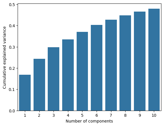
First we can analyze the amount of variance explained for the first 10 components. The first components seem to explain about 30% of the variance. That is quite a lot of unexplained variance, however, the components after that seem to contribute relative little. Lets stay with the first two components.

import matplotlib.pyplot as plt
S2=S*S
expl_var = np.cumsum(S2/sum(S2))
ax = sns.barplot(y=list(expl_var)[:10],x=list(range(1,11)))
ax.set(xlabel='Number of components', ylabel='Cumulative explained variance');

First we plot the Sample-specific vectors. These illustrate the linear combinations of genes that explains the variance of the genes. First one describes the most, the second explains most of the variance when the variance of the first gene-combination is removed. Here we only explore the first two component, but one could plot the other ones as well.

transformed_patients = pd.DataFrame(data=Vt[0:2,:].T,columns=["Sample-specific 1","Sample-specific 2"],index=list(lusc.columns) + list(luad.columns))
transformed_patients["Set"]= (["LUSC" for _ in lusc.columns]+["LUAD" for _ in luad.columns])

sns.set(rc={'figure.figsize':(10,10)})
sns.set_style("white")
#sns.set_context("talk")

sns.lmplot(x="Sample-specific 1",y="Sample-specific 2", hue='Set', data=transformed_patients, fit_reg=False)

<seaborn.axisgrid.FacetGrid at 0x7fe0e47561d0>

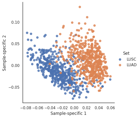
Here we see a non-complete separation of the patients based on their two first sample-specific effects. This means that the patients gene expression differ and that diference is covered by the first two principal components.

Lets explore which genes that are most reponsible for that difference. We can do so by investigating their Gene-specific vectors.

transformed_genes=pd.DataFrame(data=U[:,0:2], index = combined.index, columns = ["Gene-specific 1","Gene-specific 2"])
sns.lmplot(x="Gene-specific 1", y="Gene-specific 2", data=transformed_genes, fit_reg=False)

<seaborn.axisgrid.FacetGrid at 0x7fe09ca15cd0>

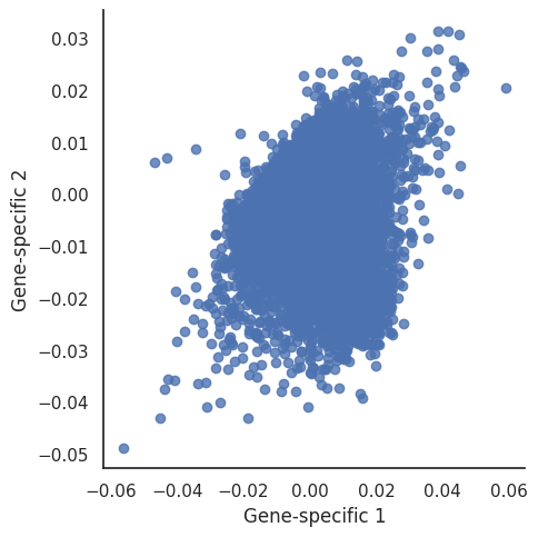
The genes pointing in a positive direction for the two components are:

transformed_genes.idxmax(axis=0)

Gene-specific 1    SFTPB
Gene-specific 2     RGL3
dtype: object

The genes pointing in a negative direction for the two components are:

transformed_genes.idxmin(axis=0)

Gene-specific 1    KRT17
Gene-specific 2    KRT17
dtype: object

KRT17 seems to be important for both Gene-specific vector 1 and 2. This is possible since KRT17 is a known cancer related gene. At this point of the analysis, it is not fully clear what the biological interpretation of PC2 is. From the sample specific effects plot, it is however clear that PC1 seem to capture a large part of the difference beween the LUAD and LUSC samples.

Note that based on this analysis only can speculate about what makes up this difference. The differences could stem from actual differences in the cancer biology of the tumors, but it could equally well be due to technical problems, such as batch effects stemming from differences in sample treatments.