6. Classification#
In regression, we typically aim to predict a continuous outcome (like a numerical value). However, we can extend the same concepts of regression to classification tasks, where the goal is to predict a discrete class label. By using specific target values (like \(y = \pm 1\)), we can transform regression into a method for classifying data.
In this chapter, we’ll explore how regression-based techniques can be adapted to solve classification problems.
6.1. The Concept of Classification with Regression#
In classification, the target variable \(y_i\) represents the class label. Common encodings for binary classification are signed labels (\(y_i \in \{-1, +1\}\)), indicator labels (\(y_i \in \{0, 1\}\)), or boolean labels (\(y_i \in \{true, false\}\)).
In this chapter, we’ll primarily use the signed labels \(y_i \in \{-1, +1\}\), but we’ll note where conversions are necessary.
6.2. Classification Loss Functions#
When applying regression techniques to classification, the choice of loss function is critical. In regression, we typically minimize the sum of squared residuals, but in classification, we use loss functions that are designed to penalize misclassifications proportional to how much the predictor insists on the incorrect prediction. Below are three common loss functions used in classification tasks:
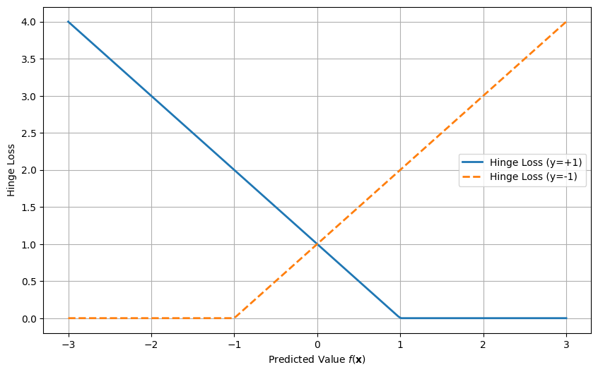
6.2.1. Hinge Loss (Used in Support Vector Machines)#
The hinge loss is commonly used in support vector machines (SVMs) that we will use in a subsequent chapter and is defined as:
This loss penalizes any data points where the predicted value \(f(\mathbf{x}_i)\) does not match the true label \(y_i\). If \(y_i f(\mathbf{x}_i) \geq 1\), the prediction is correct and there is no penalty. If \(y_i f(\mathbf{x}_i) < 1\), there is a penalty proportional to the misclassification.
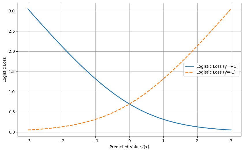
6.2.2. Logistic Loss (Used in Logistic Regression)#
The logistic loss is used in logistic regression and is defined as:
This loss function provides a smooth gradient and penalizes incorrect predictions by increasing the loss for large errors. The form above assumes signed labels \(y_i\in\{-1,+1\}\) and treats \(f(\mathbf{x}_i)\) as a real-valued score.
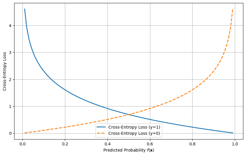
6.2.3. Cross-entropy loss#
The probably most used loss function for classification tasks is cross-entropy loss. Here we use indicator labels, i.e. \(y=1\) or \(y=0\). This loss function measures the difference between the predicted probabilities and the actual class labels. It is defined as:
For the mathematically inclinded reader, this is the negative log‑likelihood of a Bernoulli model, so minimizing it corresponds to maximum likelihood estimation for probabilistic predictions.
6.3. Classification Example: Logistic Regression#
Let’s look at a simple example where we use the concepts of regression to perform a classification task. In logistic regression, we aim to model the probability that a given data point belongs to class \(+1\) or class \(-1\).
The logistic function, also called the sigmoid function, is used to map the output of the linear function \(f(\mathbf{x})\) to a probability between 0 and 1:
Where \(f(\mathbf{x}_i) = \mathbf{x}_i^\top \beta\) is the linear function that we optimize. The logistic loss function is then minimized to find the best-fitting model.
6.4. Optimizing the Model for Classification#
To solve the classification task, we follow the same procedure used in regression:
Define a loss function: For classification, this could be the hinge loss or logistic loss.
Optimize the loss function: We minimize the loss function using methods like gradient descent or optimization tools.
Make predictions: After fitting the model, we predict the class label based on the sign of \(f(\mathbf{x})\).
6.4.1. Example of Logistic Regression in Code#
import numpy as np
import seaborn as sns
import matplotlib.pyplot as plt
from scipy.optimize import minimize

sns.set_style("whitegrid")

# Generate a simple dataset from two separate distributions
np.random.seed(0)

# Class +1 examples: centered at (0.5, 0.5)
X_pos = np.random.randn(50, 2) + 0.5
y_pos = np.ones(50)

# Class -1 examples: centered at (-0.5, -0.5)
X_neg = np.random.randn(50, 2) - 0.5
y_neg = -np.ones(50)

# Combine the datasets
y = np.hstack([y_pos, y_neg])
X = np.vstack([X_pos, X_neg])
X = np.hstack([X, np.ones((X.shape[0], 1))])  # Add intercept term

# Note: this example encodes labels as +1 and -1 (signed labels).
# If you prefer 0/1 labels for probability-based losses, convert via:
#   y01 = (y_signed + 1) / 2

# Sigmoid function
def sigmoid(z):
    return 1 / (1 + np.exp(-z))

# Logistic loss function
def logistic_loss(beta, X, y):
    z = X @ beta
    return np.sum(np.log(1 + np.exp(-y * z)))

# Initial guess for beta (weights)
initial_beta = np.zeros(X.shape[1])

# Minimize the logistic loss
result = minimize(logistic_loss, initial_beta, args=(X, y), method='BFGS')
optimized_beta = result.x

# Generate a grid of values for plotting the decision boundary
x1_range = np.linspace(X[:, 0].min() - 1, X[:, 0].max() + 1, 100)
x2_range = np.linspace(X[:, 1].min() - 1, X[:, 1].max() + 1, 100)
x1_grid, x2_grid = np.meshgrid(x1_range, x2_range)

# Compute the logistic regression decision boundary (p = 0.5)
z = optimized_beta[0] * x1_grid + optimized_beta[1] * x2_grid + optimized_beta[2]
probability = sigmoid(z)

# Create a plot with the data points and decision boundary
plt.figure(figsize=(8, 6))

# Plot the probability gradient
contour_plot = plt.contourf(x1_grid, x2_grid, probability, levels=50, cmap='coolwarm', alpha=0.7)

# Scatter plot of the dataset with class labels
sns.scatterplot(x=X[:, 0], y=X[:, 1], hue=y, palette="coolwarm", s=60, edgecolor='k')


# Add the decision boundary (p = 0.5)
# plt.contour(x1_grid, x2_grid, probability, levels=[0.5], colors='black', linestyles='--')

plt.xlabel("Feature 1")
plt.ylabel("Feature 2")
plt.grid(True)
# Add colorbar showing the predicted probability
plt.colorbar(contour_plot, label="Predicted Probability (Class +1)")

plt.show()
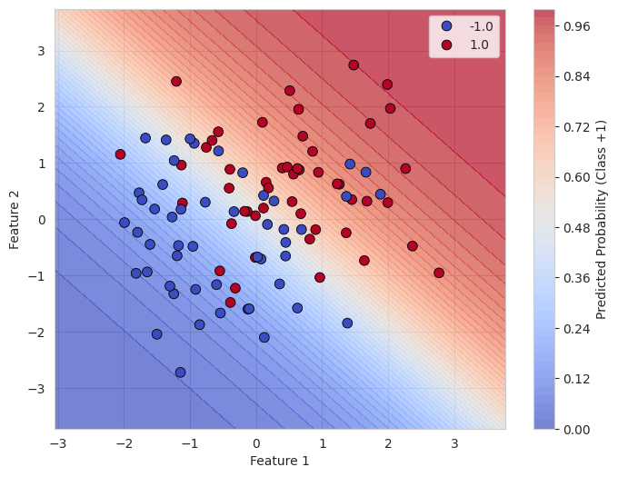
In this example:
Logistic Loss is minimized to fit a classification model.
The model predicts class labels \(y = \pm 1\), based on the sign of \(f(\mathbf{x})\).
The classification accuracy is calculated by comparing the predicted labels with the actual labels.