13. Multiple Hypothesis Corrections#
13.1. Introduction#
In high-throughput biology, analysis often involves testing a large number of hypotheses simultaneously. This is common in fields like genomics, transcriptomics, and proteomics, where experiments might involve thousands of genes or proteins being tested for associations with a condition or trait. A key challenge here is multiple hypothesis testing: when many tests are conducted, the probability of obtaining false positives increases because even a small chance of error for each test can accumulate across thousands of tests, resulting in a substantial number of false discoveries.
To understand this, imagine testing 1,000 hypotheses with a significance threshold (\(\alpha\)) of 0.05. If the null hypothesis is true for all these tests, we would still expect about 5% of them, or 50 tests, to be significant simply by chance. Without any correction for multiple comparisons, the results are prone to contain many false positives, reducing the reliability of the conclusions drawn from the data.
Multiple hypothesis correction methods are crucial for controlling error rates and ensuring that the reported results are genuinely significant and not just due to random variation. Different correction techniques control different types of error rates, such as the Family-Wise Error Rate (FWER) or the False Discovery Rate (FDR), which help us balance the trade-off between sensitivity (finding true effects) and specificity (avoiding false positives).
Both FWER and FDR are statements about the significant findings—the hypotheses that we conclude as positive results. The main objective is to ensure that the reported set of significant findings is as reliable as possible. In other words, these error rates help us control the proportion of false positives within our results, thus increasing our confidence in the findings that fall below the chosen significance threshold.
13.1.1. Bonferroni Correction#
The Bonferroni correction is one of the simplest and most conservative methods for controlling the Family-Wise Error Rate (FWER). The FWER is the probability of making at least one false positive among all the hypotheses tested. The Bonferroni correction aims to reduce the chance of any false positives by adjusting the significance threshold for each individual test.
Summary: The Bonferroni correction is simple and effective for controlling false positives but can be overly conservative, especially when the number of tests is large, leading to a loss of statistical power.
The Bonferroni method works as follows:
Given a significance level \(\alpha\), divide it by the number of hypotheses \(m\) being tested to obtain the adjusted significance level:
Conduct each individual hypothesis test using this adjusted significance level \(\alpha_{\text{adjusted}}\). If a \(p\) value is less than \(\alpha_{\text{adjusted}}\), the corresponding hypothesis is considered significant.
By using the Bonferroni correction, we control the probability of making at least one false positive across all the tests, thus providing stringent control of the error rate. However, this method can be overly conservative, especially with a large number of hypotheses, leading to a higher chance of missing true effects (i.e., a loss of statistical power).
13.1.2. Calculating the Upper Bound of the False Discovery Rate with the Benjamini-Hochberg Procedure#
The Benjamini-Hochberg (BH) procedure is a popular method for controlling the False Discovery Rate (FDR), which is the expected proportion of null among the \(p\) values below treshold. I.e. the fraction of false posives among the \(p\) values we call as significant. Unlike more conservative approaches like the Bonferroni correction, which aims to eliminate all false positives at the cost of potentially missing true effects, the BH method balances sensitivity and specificity by controlling the rate of false discoveries.
The BH procedure involves ranking the \(p\) values from all the tests in ascending order. Let’s denote these ordered \(p\) values as \(p_{(1)}, p_{(2)}, \dots, p_{(m)}\), where \(m\) is the total number of hypotheses. The method works as follows:
Rank all the \(p\) values such that \(p_{(1)} \le p_{(2)} \le \dots \le p_{(m)}\).
Choose a desired FDR level, denoted as \(q\).
For each \(p\) value \(p_{(i)}\), calculate the threshold value:
where \(i\) is the rank of the \(p\) value and \(m\) is the total number of hypotheses. 4. Find the largest \(i\) for which \(p_{(i)} \le \frac{i}{m} \times q\). Accept all hypotheses with \(p\) values less than or equal to \(p_{(i)}\).
Summary: The Benjamini-Hochberg procedure is less conservative than Bonferroni, providing a balance between controlling false positives and finding true effects, making it more suitable when a moderate number of false positives is acceptable.
By using this approach, the BH procedure ensures that the expected proportion of false discoveries is controlled at the desired level \(q\), allowing us to draw more reliable conclusions while still maintaining a reasonable sensitivity to detect true effects.
13.1.3. Calculating q-values with Storey’s Method#
Storey introduced an alternative to the Benjamini-Hochberg procedure for controlling the False Discovery Rate (FDR), known as the q-value approach. The q-value can be thought of as the FDR analogue of the \(p\) value; it provides a measure of significance that directly incorporates the concept of multiple hypothesis testing, offering an estimate of the proportion of false positives incurred when calling a particular test significant.
Storey’s method (as well as the Benjamini-Hochberg procedure) is founded on the understanding that \(p\) values arise from one of two possible realities: they are generated either under the null hypothesis (\(H_0\)) or under the alternative hypothesis (\(H_1\)). Under \(H_0\), \(p\) values are uniformly distributed, indicating no real effect, and their values reflect random variation. In contrast, under \(H_1\), \(p\) values tend to be smaller, indicating evidence against the null and suggesting a true effect. These methods work by distinguishing between these two underlying distributions of \(p\) values to control the error rate (such as FDR) while balancing the discovery of true positives. The fundamental assumption is that the observed set of \(p\) values is a mixture of those generated by true null hypotheses and those generated by true alternatives, and effective control of FDR hinges on accurately estimating the proportions of each. Unlike for the Benjamini-Hochberg procedure, we here estimate a fraction, \(\pi_0\), of all the evaluated \(p\) values that are null statistics.
Storey’s procedure calculates the total number of features considered significant by counting all \(p\) values below a threshold \(t\). The number of nulls below this threshold, is estimated as \(\pi_0 m t\), where \(\pi_0\) is the estimated fraction of null hypotheses, \(m\) is the total number of hypotheses, and \(t\) is the chosen threshold. This could be done as there is expected to be \(\pi_0 m\) nulls, uniformly distributed between, 0 and 1, and a fraction \(t\) of them is expected to be under threshhold.
The proportion of null statistics \(\pi_0\) is estimated by a procedure of its own. If all hypotheses were null, we would expect approximately \(m(1 - \lambda)\) \(p\)-values above a threshold \(\lambda\). However, the presence of true alternative hypotheses results in fewer \(p\)-values above \(\lambda\), so the proportion of values above the threshold provides an estimate of \(\pi_0\), the proportion of true null hypotheses. As \(\lambda\) approaches 1, this estimate contains fewer alternative \(p\)-values but the estimate also more variable, so a smoothing function (spline) is applied to stabilize the estimate by evaluating it at \(\lambda = 1\).
Here is how Storey’s q-value procedure works, as described by Storey & Tibshirani:
Order the \(p\) values: Let \(p_{(1)} \le p_{(2)} \le \dots \le p_{(m)}\) be the ordered \(p\) values. This ordering of \(p\) values ranks the features in terms of their evidence against the null hypothesis, with lower \(p\) values suggesting stronger evidence.
Estimate \( \pi_0 \) for a range of \( \lambda \) values:
For a range of \( \lambda \) values, such as \( \lambda = 0, 0.05, 0.10, \dots, 0.95 \), calculate the proportion of \(p\) values greater than \(\lambda\):
\[\hat{\pi}_0(\lambda) = \frac{|\{ p_i > \lambda \}|}{m (1 - \lambda)}\]where \(|\{ p_i > \lambda \}|\) represents the count of \(p\) values greater than \(\lambda\), and \(m\) is the total number of hypotheses.
Fit a natural cubic spline to estimate \( \pi_0 \):
Let \( \hat{f} \) be the natural cubic spline fitted to \(\hat{\pi}_0(\lambda)\) as a function of \(\lambda\). The final estimate of \( \pi_0 \) is given by evaluating the spline at \( \lambda = 1 \):
\[\hat{\pi}_0 = \hat{f}(1)\]A spline is a piecewise polynomial function that is used to create smooth curves through a set of data points. Essentially, it fits multiple polynomial functions between segments of the data to form a single, continuous curve that is both flexible and smooth. The advantage of using splines is that they help create a smooth approximation without oscillations, especially when dealing with complex or unevenly spaced data. For more details, you can check out the Wikipedia page on splines.
Estimate the FDR for each \(p\) value:
The FDR for each treshold at the ordered \(p\) value \(p_{(i)}\), by considering the estimated number of significant null statistics, \(\hat{\pi}_0 m p_{(i)}\), divided by the number of \(p\)-values below or at a threshold, \(t=p_{(i)}\).
\[\hat{\rm FDR}(t=p_{(i)}) = \left( \frac{\hat{\pi}_0 m p_{(i)}}{i} \right)\]Ensure monotonicity:
Assign \(\hat{q}_{(m)} = \hat{\pi}_0\)
For \( i = m - 1, m - 2, \dots, 1 \), update the q-values to ensure they are monotonically increasing:
\[\hat{q}_{(i)} = \min(\hat{\rm FDR}(t=p_{(i)}), \hat{q}_{(i+1)})\]This ensures that higher \(p\) values do not end up with lower q-values, maintaining logical consistency in the significance estimates.
Summary: Storey’s method provides a more flexible and often less conservative approach to controlling the FDR compared to traditional methods. By adapting the estimate of \(\pi_0\), Storey’s method can achieve more powerful statistical inference, particularly when many of the hypotheses are expected to be null. It should be noted that Storeys procedure gives gives similar estimates as Benjamini-Hochberg if we set \(\pi_0=1\), i.e. the Storey procedure is less conservative than Benjamini-Hochberg for most situations.
Note
Alternative Procedure for \(\pi_0\) Estimation
In steps 2 and 3 of Storey’s method for estimating \(\pi_0\), an alternative approach involves the use of bootstrapping to refine the estimate. The goal of estimating \(\pi_0\) is to determine the proportion of true null hypotheses, which is crucial for accurately controlling the False Discovery Rate (FDR). The procedure described below leverages bootstrapping to obtain a more robust and potentially less biased estimate of \(\pi_0\).
The alternative procedure for estimating \(\pi_0\) can be broken down as follows:
Lambda Selection: Instead of fitting a natural cubic spline to the estimates of \(\pi_0\) for different values of \( \lambda \), this approach first selects a range of \( \lambda \) values, evenly spaced between a small value and a maximum value, typically \( \lambda = 0.95 \). These \( \lambda \) values help determine how many of the \(p\) values exceed the threshold, giving an initial estimate of \(\pi_0\).
Initial Estimation: For each value of \( \lambda \), the number of \(p\) values greater than \( \lambda \) is counted. The initial estimate of \(\pi_0\) is calculated using:
where \( W(\lambda) \) is the count of \(p\) values greater than \( \lambda \), and \( n \) is the total number of \(p\) values. The smallest of these estimates is retained as an initial \(\pi_0\) estimate.
Bootstrapping for Stability: To obtain a more stable and reliable estimate, the procedure employs bootstrapping. Bootstrapping involves resampling the \(p\) values with replacement multiple times (e.g., 100 times) to generate different bootstrap samples. For each bootstrap sample, \(\pi_0\) is re-estimated for all \( \lambda \) values. The mean squared error (MSE) is then calculated for each \( \lambda \), comparing the bootstrap estimates with the initial minimum estimate.
Final \(\pi_0\) Estimate: The final \(\pi_0\) estimate is selected as the value that minimizes the MSE across the bootstrap iterations, resulting in an estimate that is less sensitive to fluctuations in the data and less prone to bias.
This bootstrapping-based approach helps improve the accuracy of the \(\pi_0\) estimate, particularly when the proportion of true null hypotheses is not easily identifiable. By using multiple resamples, the estimate becomes more robust against random variations, leading to more reliable control of the FDR.
This approach provides a more adaptive and refined way to estimate \(\pi_0\), enhancing the reliability of downstream FDR calculations and hypothesis testing results.
13.1.4. Illustration of q-value calculations#
Below is a simulation of \(p\) value distributions for multiple hypotheses, showcasing the challenge of distinguishing true effects from random variation:
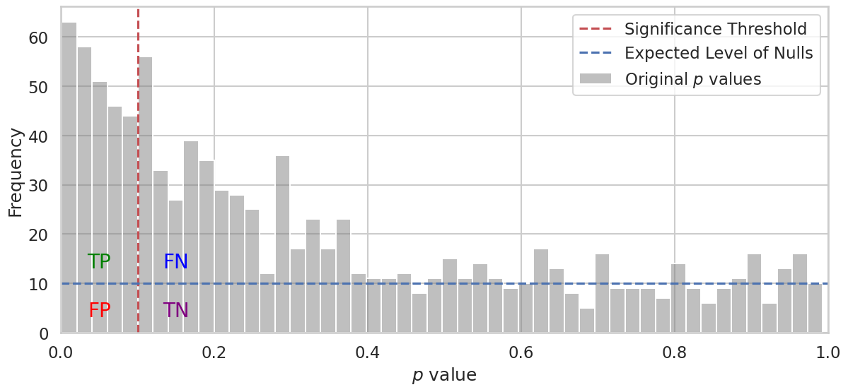
In the plot above, we simulate \(p\) values for a large number of hypotheses (1,000 in this case). Half of these hypotheses represent nulls (meaning there is no effect), while the other half represent alternative hypotheses (meaning there is a true effect).
True Null Hypotheses: The \(p\) values for the nulls are generated from a uniform distribution between 0 and 1. This means that \(p\) values are evenly spread across this range, representing the random chance of seeing a particular \(p\) value when there is actually no effect. The \(p\) values under the null hypothesis are uniformly distributed because they represent the probability of observing data as extreme as the actual result, assuming the null hypothesis is true. When the null hypothesis is true, each outcome has an equal chance of occurring, meaning that any \(p\) value between 0 and 1 is equally likely. This uniform distribution reflects the lack of any real effect, where the observed data could be due to random chance alone.
Alternative Hypotheses: The \(p\) values for the alternative hypotheses are concentrates more \(p\) values towards smaller values, particularly near zero. This is because, when there is a true effect, the data is less likely to be generated under the null hypothesis, making the resulting \(p\) values low. In other words, small \(p\) values provide stronger evidence against the null hypothesis, indicating that the observed effect is unlikely to be due to random chance alone.
The accumulation of \(p\) values towards 0 for the alternative hypotheses is an indication of true effects being detected in the data. When a true effect exists, we should be able to reject the null hypothesis confidently, resulting in smaller \(p\) values.
13.1.4.1. Finding a Threshold for Statistical Significance#
In hypothesis testing, we want to determine a threshold that can help us identify true positives (TP) while minimizing false positives (FP). In the plot, we draw a vertical red line representing a threshold above which we do not consider the hypothesis significant.
Left of the threshold: The hypothesies with \(p\) values below (or at) threshold are called significant. We want to find true positives (TP), which are genuine effects that we correctly identify. However, we may also mistakenly identify false positives (FP), which are hypotheses that are actually null but end up below the threshold due to random variation.
TP (True Positives): These are significant findings that correspond to real effects, i.e. alternative hypotheses below treshold. We hope to see many of these as posible.
FP (False Positives): These are findings found significant, even though they are null, i.e. null hypotheses below treshold.
Right of the threshold: The hypothesies with \(p\) values above threshold are called not significant. Here we have true negatives (TN) and false negatives (FN).
FN (False Negatives): These are true effects (alternative hypotheses) that we fail to detect because their \(p\) values are above our significance threshold. A high number of FNs means that our test lacks sensitivity.
TN (True Negatives): These are null hypotheses found not significant.
13.1.4.2. False Discovery Rate (FDR)#
When applying a significance threshold, we aim to find a balance between detecting true effects and minimizing errors. Specifically, we want to find a threshold that provides a good proportion of true findings while controlling the False Discovery Rate (FDR).
The FDR is defined as the expected proportion of false positives among all rejected null hypotheses. This is approximately:
In other words, we want to keep the number of false positives relative to the total number of findings low, while still identifying as many true effects as possible. Setting the right significance threshold helps to control the FDR, allowing us to make reliable discoveries without overstating our results.
The annotations in the plot—TP, FP, FN, and TN—highlight the different outcomes relative to the threshold. This visualization helps us understand the impact of different choices of significance level on our findings and the trade-offs between sensitivity (detecting true positives) and specificity (avoiding false positives).