


Why we need a ground truth
In the previous chapter we estimated false discovery rates. The B6 against B6 comparison let us check that the procedure reports nothing when every gene follows the null hypothesis, but such a null experiment only checks the null side: it contains no true findings, and in the comparison of the two strains we do not know which genes are truly differentially expressed. A procedure that reports makes a promise about the long run frequency of errors among its findings, and that promise should be testable.
A spike-in experiment, which contains known true positives as well as true nulls, lets us test it. One prepares a complex but constant biological background, and adds a small number of foreign proteins at concentrations chosen, and therefore known, by the experimenter. Only the spiked-in proteins should differ between the samples. We can then run a complete differential abundance analysis and afterwards count how many of our findings were actually changed. The fraction of errors among the findings is the false discovery proportion (FDP),
which is what , and hence , is trying to predict. The FDR is an expectation over hypothetical repetitions of the experiment; the FDP is a number we can read off a single data set, if we know the truth.
The iPRG 2015 spike-in study
We will use the benchmark set of the ABRF Proteome Informatics Research Group, described by Choi et al., J. Proteome Res. 2017, and deposited at MassIVE under accession MSV000079843.
A tryptic digest of a Saccharomyces cerevisiae lysate was used as background, identical in all samples. Into it six proteins were spiked at four different combinations of concentrations, giving four sample groups, each analysed in triplicate on a Q-Exactive instrument: twelve LC-MS/MS runs in total. Table 1 of Choi et al. lists the amounts, in fmol per injection:
| Name in the data set | Spiked protein | Condition 1 | Condition 2 | Condition 3 | Condition 4 |
|---|---|---|---|---|---|
| VAC2_YEAST | Ovalbumin (chicken) | 65 | 55 | 15 | 2 |
| ISCB_YEAST | Myoglobin (horse) | 55 | 15 | 2 | 65 |
| SFG2_YEAST | Phosphorylase b (rabbit) | 15 | 2 | 65 | 55 |
| UTR6_YEAST | β-Galactosidase (E. coli) | 2 | 65 | 55 | 15 |
| PGA4_YEAST | Serum albumin (bovine) | 11 | 0.6 | 10 | 500 |
| ZRT4_YEAST | Carbonic anhydrase (bovine) | 10 | 500 | 11 | 0.6 |
None of the six spiked proteins is a yeast protein. In the data set they carry disguised, yeast-like names and accession numbers, so that the participants in the study could not spot them by looking at the protein list. Every other protein in the experiment is a yeast protein and should, by construction, be unchanged.
We start from the protein-level table that the MSstats pipeline produces after summarising the Skyline peptide intensities into one log intensity per protein and run.
Notebook Cell
# When the page runs in the browser (JupyterLite), we install seaborn, and fetch the files that this chapter reads from the book's repository
import sys
if sys.platform == "emscripten":
    import os
    import micropip
    await micropip.install(["seaborn", "pyodide-http"])
    import pyodide_http
    pyodide_http.patch_all()
    from urllib.request import urlretrieve
    repo = "https://raw.githubusercontent.com/statisticalbiotechnology/dsbook/main/dsbook/"
    for remote, local in [("common/qvalue.py", "../common/qvalue.py"),
                          ("statistics/data/iprg2015_protein_runsummary.csv", "data/iprg2015_protein_runsummary.csv")]:
        if not os.path.exists(local):
            os.makedirs(os.path.dirname(local), exist_ok=True)
            urlretrieve(repo + remote, local)
import pandas as pd
import numpy as np
from scipy.stats import ttest_ind
import sys
IN_COLAB = 'google.colab' in sys.modules
if IN_COLAB:
![ ! -f "dsbook/README.md" ] && git clone https://github.com/statisticalbiotechnology/dsbook.git
my_path = "dsbook/dsbook/statistics/"
else:
my_path = "./"
sys.path.append(my_path + "../common/") # Read the local module for q value calculations
import qvalue
# Protein-level run summary of the iPRG2015 study (MassIVE MSV000079843), as produced by
# MSstats from the Skyline output. Reshaped to a wide table from the teaching copy in
# https://github.com/ZenBrayn/asms_2020_fall_workshop (exercises/day3_basic_stat/iPRG_example_runsummary.csv)
iprg = pd.read_csv(my_path + "data/iprg2015_protein_runsummary.csv", index_col=0)
iprg = iprg.dropna() # keep proteins quantified in all twelve runs
spiked = iprg["Spikein"] # the ground truth: True for the six spiked proteins
intensity = iprg.drop(columns="Spikein")
print(intensity.shape, "proteins x runs, of which", spiked.sum(), "are spiked in")
intensity.head()(3025, 12) proteins x runs, of which 6 are spiked in
The twelve columns are named after the sample group and the technical replicate, which makes the design easy to recover.
design = pd.DataFrame([c.split("_") for c in intensity.columns],
                      columns=["Condition", "Replicate"], index=intensity.columns)
design.TThe design is visible in the data
Before doing any statistics we look at the quantities themselves. For every protein we subtract its own mean log intensity, putting all proteins on a comparable scale, and plot the profile over the four conditions.
import matplotlib.pyplot as plt
import seaborn as sns
sns.set_style("whitegrid")
sns.set_context("talk")

condition_means = intensity.T.groupby(design["Condition"]).mean().T   # protein x condition
centered = condition_means.sub(condition_means.mean(axis=1), axis=0)

fig, ax = plt.subplots(figsize=(9, 6))
rng = np.random.default_rng(1)
background = centered.loc[~spiked]
for prot in rng.choice(background.index, 200, replace=False):
    ax.plot(range(4), background.loc[prot], color="grey", alpha=0.15, lw=1)
for prot in centered.loc[spiked].index:
    ax.plot(range(4), centered.loc[prot], marker="o", lw=3, label=prot.split("|")[2])
ax.set_xticks(range(4), ["Cond 1", "Cond 2", "Cond 3", "Cond 4"])
ax.set_ylabel("centered $\\log_2$ intensity")
ax.legend(fontsize=11, ncol=3, loc="upper center", bbox_to_anchor=(0.5, 1.22));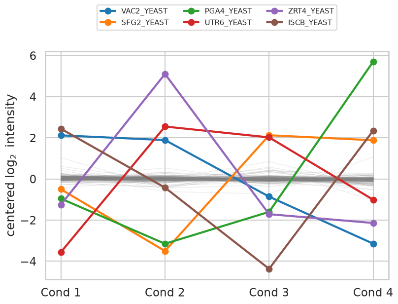
The grey band of background proteins is essentially flat — 95% of them vary by less than a factor of two between the extreme conditions — while the six coloured profiles swing by factors of forty to five hundred, following the concentration table above.
Differential abundance between two conditions
We now perform the analysis we would have performed without knowing the truth: a test of every protein between condition 1 and condition 2, as in the differential expression chapter. One detail differs. With only three replicates per group we use the pooled-variance test rather than Welch’s, since Welch’s correction buys robustness against unequal variances at a price in degrees of freedom that we cannot afford at .
def compare(cond_a, cond_b):
    """Two sample t test of every protein between two sample groups."""
    a = intensity.loc[:, design["Condition"] == cond_a]
    b = intensity.loc[:, design["Condition"] == cond_b]
    p = ttest_ind(a, b, axis=1)[1]
    return pd.DataFrame({"p": p,
                         "log_FC": b.mean(axis=1) - a.mean(axis=1),
                         "Spikein": spiked}, index=intensity.index)

results = compare("Condition1", "Condition2")
results.sort_values("p").head(8)The value histogram of the background proteins is the diagnostic that the null distribution behaves. If the yeast proteins really are unchanged, and the test is correctly calibrated, their values should be uniformly distributed on .
fig, ax = plt.subplots(figsize=(9, 5))
sns.histplot(x=results.loc[~results["Spikein"], "p"], bins=20, stat="density", ax=ax,
             color="steelblue", label="yeast background (true nulls)")
ax.axhline(1.0, color="black", ls="--", lw=2)
for p in results.loc[results["Spikein"], "p"]:
    ax.plot([p], [0.06], marker="^", ms=14, color="firebrick", clip_on=False)
ax.set_xlim(0, 1); ax.set_xlabel("$p$"); ax.legend(fontsize=13)
ax.set_title("red triangles: the six spiked proteins", fontsize=14);
print("fraction of background proteins with p < 0.05:",
      round((results.loc[~results["Spikein"], "p"] < 0.05).mean(), 3))
fraction of background proteins with p < 0.05: 0.034
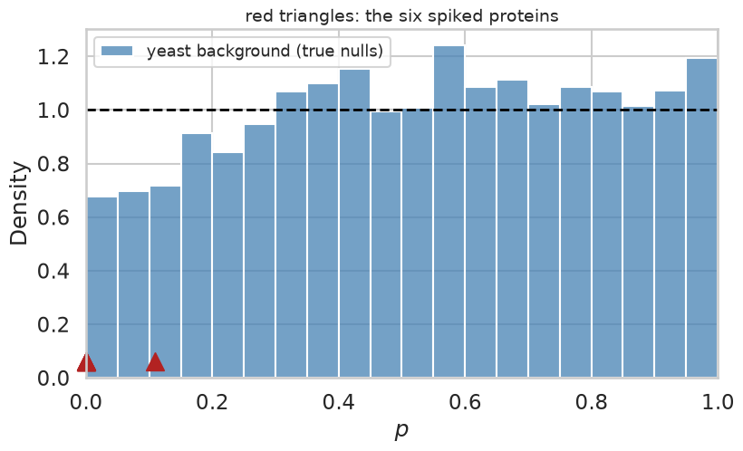
The histogram is close to flat, if somewhat depleted near zero, and the fraction of background proteins below is a little under the 5% that a uniform null would give. The background is a proper — indeed mildly conservative — null. Five of the six spiked proteins sit at the extreme left edge. The sixth is VAC2, which was spiked at 65 and 55 fmol in the two conditions — a genuine but only 1.2-fold difference that three replicates cannot resolve. It will end up as a false negative, but not one that any method could reasonably be expected to avoid.
values
We estimate and the values with the same bootstrap procedure as in the
previous chapter, here imported from the book’s common module rather than
retyped.
np.random.seed(0)   # the pi_0 estimate is based on bootstrapping
print("pi_0 estimated to", round(qvalue.estimatePi0(list(results["p"].values)), 3))
results = qvalue.qvalues(results)
results.head(8)
pi_0 estimated to 1.001
The estimate says that essentially none of the proteins are differentially abundant, which is the correct answer: 6 out of 3025 is . Contrast this with the comparison of the two mouse strains in the previous chapter, where came out at about 0.5.
The payoff: estimated FDR against the true FDP
Because we know which proteins were spiked, we can walk down the list in order of increasing value and, at every position, compute both what the procedure claims the error rate is and what it actually is.
results["FDP"] = (~results["Spikein"]).cumsum() / np.arange(1, len(results) + 1)

top = results.head(15)
fig, ax = plt.subplots(figsize=(9, 6))
ax.step(range(1, 16), top["q"], where="mid", lw=3, label="estimated $q$ value")
ax.step(range(1, 16), top["FDP"], where="mid", lw=3, ls="--", label="true FDP")
ax.set_xlabel("number of proteins accepted")
ax.set_ylabel("false discovery rate")
ax.set_ylim(0, 1); ax.legend(fontsize=13);
top[["p", "log_FC", "Spikein", "q", "FDP"]]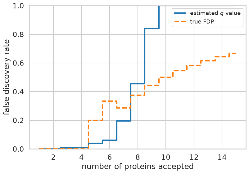
The four highest ranked proteins are all spiked, and there the value and the FDP agree at essentially zero. The first background protein enters at rank five, where the observed FDP jumps to against an estimate of 0.04. From then on the two curves track each other loosely, with the estimate rising the faster of the two: by the tenth acceptance it has already saturated at one, while the true FDP is only one half. Note also how granular the FDP is: among accepted proteins it can take only the values , and with only six true positives stays small in the interesting part of the list, so one unlucky background protein at rank five moves it by twenty percentage points. That granularity is a property of the benchmark, not of the method.
To get a less noisy picture we repeat the analysis for all six pairs of conditions and record, at a set of value thresholds, how many proteins were accepted and what fraction of them were background.
import itertools
np.random.seed(0)
thresholds = [0.01, 0.02, 0.05, 0.1, 0.2]
rows = []
for a, b in itertools.combinations(range(1, 5), 2):
    r = qvalue.qvalues(compare(f"Condition{a}", f"Condition{b}"))
    for t in thresholds:
        accepted = r[r["q"] <= t]
        if len(accepted) > 0:
            rows.append({"comparison": f"{a} vs {b}", "threshold": t,
                         "accepted": len(accepted),
                         "true positives": int(accepted["Spikein"].sum()),
                         "FDP": 1 - accepted["Spikein"].mean()})
calibration = pd.DataFrame(rows)
calibration.pivot(index="threshold", columns="comparison", values="FDP").round(2)comparisons = sorted(calibration["comparison"].unique())
# many comparisons share an FDP of exactly zero, so nudge them apart horizontally
jitter = {c: 1 + (i - 2.5) * 0.035 for i, c in enumerate(comparisons)}
calibration["x"] = calibration["threshold"] * calibration["comparison"].map(jitter)
fig, ax = plt.subplots(figsize=(7.5, 7))
sns.scatterplot(data=calibration, x="x", y="FDP", hue="comparison", s=120, ax=ax)
diagonal = np.geomspace(0.008, 0.26, 50)
ax.plot(diagonal, diagonal, color="black", ls="--", lw=2)
ax.set_xscale("log"); ax.minorticks_off()
ax.set_xticks(thresholds, [str(t) for t in thresholds])
ax.set_xlabel("estimated FDR ($q$ value threshold)")
ax.set_ylabel("true FDP")
ax.set_xlim(0.008, 0.28); ax.set_ylim(-0.03, 1.0)
ax.legend(fontsize=11, title="conditions");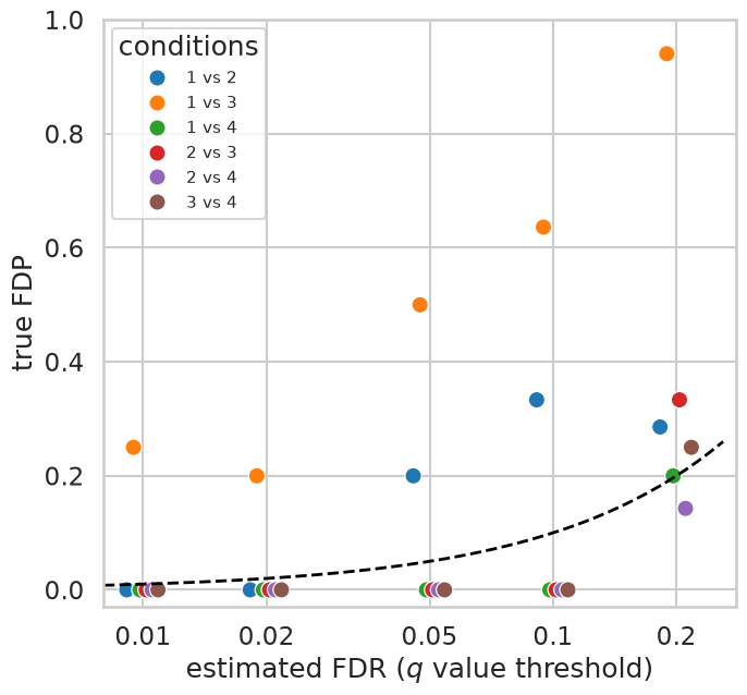
Points on the dashed line are perfectly calibrated, points below it conservative and points above it anti-conservative. At the strictest settings the procedure makes almost no mistakes: five of the six comparisons have an FDP of exactly zero at , and four of them still do at . Further out the points scatter around and mostly above the line, with FDPs between 0.14 and 0.33 at . Part of that drift is unavoidable arithmetic rather than a real bias — one false discovery among five accepted proteins is already an FDP of 0.2, so a benchmark with six true positives simply cannot resolve an FDR of 0.05.
Condition 1 versus 3 is the real outlier. At roughly two thirds of the accepted proteins are background, and its comes out around 0.6 — the estimator concluded that more than a third of the yeast proteins were differentially abundant. Printing and the behaviour of the background for every comparison shows where the problem lies.
np.random.seed(0)
for a, b in itertools.combinations(range(1, 5), 2):
    r = compare(f"Condition{a}", f"Condition{b}")
    bg = r.loc[~r["Spikein"], "p"]
    print(f"{a} vs {b}:  pi_0 = {qvalue.estimatePi0(list(r['p'].values)):.2f}"
          f"   background fraction with p<0.05 = {(bg < 0.05).mean():.3f}")
1 vs 2: pi_0 = 1.00 background fraction with p<0.05 = 0.034
1 vs 3: pi_0 = 0.63 background fraction with p<0.05 = 0.109
1 vs 4: pi_0 = 0.78 background fraction with p<0.05 = 0.054
2 vs 3: pi_0 = 0.91 background fraction with p<0.05 = 0.068
2 vs 4: pi_0 = 1.00 background fraction with p<0.05 = 0.034
3 vs 4: pi_0 = 0.91 background fraction with p<0.05 = 0.034
This is not a failure of the value machinery but of our assumption about the ground truth. For condition 1 versus 3 more than one in ten of the yeast proteins falls below , about twice what a uniform null would give, and the estimator is right to conclude that something is changing. The yeast background is simply not perfectly identical between those two sample groups. All four samples were made from the same yeast digest and the twelve runs were acquired in random order, but each sample was spiked separately, and with only three runs per sample, randomisation cannot fully average out drift of the instrument. Small differences in the amount of digest that ended up in each sample, or in the conditions under which its runs were acquired, leave systematic traces in the quantities. No FDR estimator can protect against a null that is not a null, and the proteins it flags are not errors of statistics but of our labelling of the truth. A benchmark tells us about the whole pipeline — sample preparation, quantification, normalisation and statistics together — not only about the last step.
What you should know after reading this chapter
You should be able to:
Describe how a spike-in experiment creates a known ground truth, and contrast the false discovery proportion (FDP), which can be read off a single data set when the truth is known, with the FDR, which is an expectation.
Calculate the FDP among the top findings of a ranked list with known truth, and explain why the FDP is so granular when a benchmark contains only a few true positives.
Interpret a calibration plot of true FDP against estimated FDR ( value threshold): points on the diagonal are calibrated, points below it are conservative and points above it are anti-conservative.
Argue that an estimated well below one, in data where almost nothing should change, points to a problem in the experiment or the pipeline (a null that is not a null) rather than in the FDR estimation.
- Choi, M., Eren-Dogu, Z. F., Colangelo, C., Cottrell, J., Hoopmann, M. R., Kapp, E. A., Kim, S., Lam, H., Neubert, T. A., Palmblad, M., Phinney, B. S., Weintraub, S. T., MacLean, B., & Vitek, O. (2017). ABRF Proteome Informatics Research Group (iPRG) 2015 Study: Detection of Differentially Abundant Proteins in Label-Free Quantitative LC–MS/MS Experiments. Journal of Proteome Research, 16(2), 945–957. 10.1021/acs.jproteome.6b00881