


Principal Component Analysis (PCA) is an unsupervised learning method that finds the axes of maximum variation in your data and projects the data onto them. In biotechnology it is used to find the major sources of variation in gene expression data, to visualize how samples relate to each other, to detect batch effects and outliers, and as a preprocessing step before clustering.
Decomposition of a matrix
From linear algebra, we know that we can multiply two vectors into a matrix.
What if we could do the opposite? I.e., given a matrix , what would be the vectors and that best represent so that ? This is, in essence, what you do with principal component analysis (PCA).
A scenario where this might be useful
In PCA, we often deal with a matrix that encapsulates multiple sources of variation. Imagine a scenario where we’re studying gene expression levels across several samples. Here, the gene expression levels might be influenced by two key factors:
Gene-Specific Effects: These are inherent to each gene, such as its baseline expression level or potential for expression. For example, some genes may generally be expressed at high levels across all conditions, while others have lower baseline expression.
Sample-Specific Effects: These capture the influence of each sample (environmental condition, patient, disease state) on gene expression. For instance, one condition might increase expression levels across many genes, while another has a weaker or even suppressive effect.
If the expression matrix is the outer product of these two effects, , then holds the gene-specific effects and the sample-specific effects.
A toy example
Let us make this concrete with 4 genes and 4 samples. Let the gene-specific effects be and the sample-specific effects . Each entry of the outer product is :
In practice we only observe , and PCA has to find the underlying factors. This toy matrix was built from a single pair of vectors, so it has rank 1: the first principal component reproduces exactly, and all further components are zero. Real data are never exactly of rank 1, and the later components then describe the variation that the first one leaves unexplained.
Scaling the components
The magnitude of a component can be moved freely between and : if we scale by a factor and by , the product stays the same. To make the decomposition unique, we scale both vectors to unit length,
and collect the whole magnitude in a scalar :
(one entry per gene) and (one entry per sample) then only give directions, while measures the strength of the component. The variance that the component explains is proportional to .
More than one principal component
Once the first component is removed from , the residuals can in turn be decomposed. The vectors and that best describe this residual matrix form the second principal component, while the original pair forms the first.
In this manner, we can derive as many principal components as there are rows or columns (whichever is smaller) in . For plotting, we usually look at the first two or three components; for further analysis, such as the clustering of single cells later in this part of the book, we often keep more.
An illustration of PCA
| Sample 1 | Sample 2 | Sample 3 | Sample | Gene specific | Gene specific | |||
|---|---|---|---|---|---|---|---|---|
| Gene 1 | ||||||||
| Gene 2 | ||||||||
| Gene 3 | ||||||||
| Gene | ||||||||
| Sample specific | ||||||||
| Sample specific |
Principal Components
PCA aims to identify the directions, or principal components, in the data that describe the most variance. These directions are essentially the new axes into which the original data is projected, and they help us gain insight into the underlying structure and patterns. The principal components are ordered such that the first principal component describes the largest possible variance, while each subsequent component describes as much of the remaining variance as possible, subject to being orthogonal to the preceding components.
The gene-specific vector and the sample-specific vector come in pairs. Together, the first few pairs give the best low-dimensional description of , in the sense that they minimize the sum of squared residuals. The two members of a pair are linked by projection:
Projecting on collapses each row (gene) of onto a single number, and gives .
Projecting on collapses each column (sample) of onto a single number, and gives .
So is, up to the scaling factor , the projection of on , and vice versa. The entries of are used as sample-specific scores, which show where each sample lies along a component, and the entries of as gene-specific loadings, which show which genes drive the component.
Dimensionality Reduction and Explained Variance
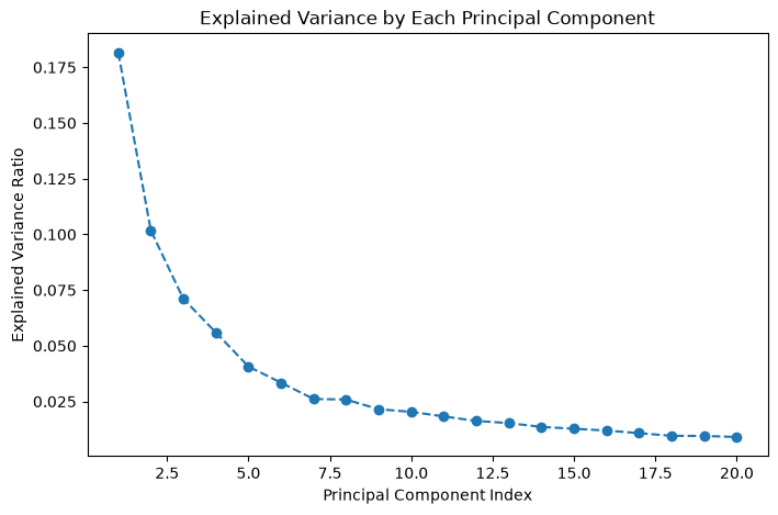
Keeping only the first few components is a form of dimensionality reduction: each sample is described by its scores on a handful of components instead of by thousands of gene expression values. The share of the total variance that a component describes is called its explained variance. It decreases from the first component onwards, and a plot of the explained variance per component, a scree plot, shows how many components are needed to capture most of the variation.
Geometrically, PCA is an affine transformation: it subtracts the mean (a translation) and rotates the data onto new axes. Keeping only the first few axes then projects the data onto a lower-dimensional subspace. Because this projection is linear, it can flatten the data but cannot unfold a curved structure.
Singular Value Decomposition (SVD)
Principal components are calculated with the singular value decomposition (SVD). Before the decomposition, the data are centered: the mean of each variable (for example, each gene’s mean expression across the samples) is subtracted, so that the components describe the variation around the mean rather than the mean itself. The SVD then decomposes the centered data matrix as
where
the columns of are the gene-specific vectors ,
the columns of are the sample-specific vectors ,
is a diagonal matrix that holds the singular values , the magnitude of each principal component pair.
Since the variance described by a component is proportional to , the fraction of the variance explained by component is . Without centering, the first component would mostly describe the mean, and this ratio would be a fraction of the sum of squares rather than of the variance.
An example of reconstruction with PCA, Eigenfaces
Notebook Cell
# When the page runs in the browser (JupyterLite), we let Python download files through the browser
import sys
if sys.platform == "emscripten":
    import micropip
    await micropip.install("pyodide-http")
    import pyodide_http
    pyodide_http.patch_all()
import matplotlib.pyplot as plt
from numpy.random import RandomState
from sklearn.datasets import fetch_olivetti_faces
from sklearn.decomposition import PCA
rng = RandomState(0)
# Load the Olivetti faces dataset
faces, _ = fetch_olivetti_faces(return_X_y=True, shuffle=True, random_state=rng)
n_samples, n_features = faces.shape
# Global centering (focus on one feature, centering all samples)
faces_centered = faces - faces.mean(axis=0)
# Local centering (focus on one sample, centering all features)
faces_centered -= faces_centered.mean(axis=1).reshape(n_samples, -1)
print("Dataset consists of %d faces" % n_samples)
# Define a base function to plot the gallery of faces
n_row, n_col = 5, 4
n_components = n_row * n_col
image_shape = (64, 64)
def plot_gallery(title, images, n_col=n_col, n_row=n_row, cmap=plt.cm.gray):
fig, axs = plt.subplots(
nrows=n_row,
ncols=n_col,
figsize=(2.0 * n_col, 2.3 * n_row),
facecolor="white",
constrained_layout=True,
)
fig.set_constrained_layout_pads(w_pad=0.01, h_pad=0.02, hspace=0, wspace=0)
fig.set_edgecolor("black")
fig.suptitle(title, size=16)
for ax, vec in zip(axs.flat, images):
vmax = max(vec.max(), -vec.min())
im = ax.imshow(
vec.reshape(image_shape),
cmap=cmap,
interpolation="nearest",
vmin=-vmax,
vmax=vmax,
)
ax.axis("off")
fig.colorbar(im, ax=axs, orientation="horizontal", shrink=0.99, aspect=40, pad=0.01)
plt.show()
# Create a PCA model and fit it to the centered faces
print("Fitting PCA model to faces dataset...")
pca = PCA(n_components=n_components, random_state=rng)
pca.fit(faces_centered)
# Extract the eigenfaces (principal components)
eigenfaces = pca.components_
# Plot the first n_components eigenfaces
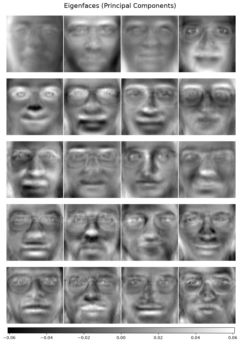
plot_gallery("Eigenfaces (Principal Components)", eigenfaces[:n_components])
# Project the original faces onto the PCA components to get their low-dimensional representation
faces_pca_projection = pca.transform(faces_centered)
# Reconstruct the faces using the PCA projection
faces_reconstructed = pca.inverse_transform(faces_pca_projection)
# Plot a gallery of original and reconstructed faces for comparison
plot_gallery("Original Centered Faces", faces_centered[:4*5],5,4)
plot_gallery("Reconstructed Faces", faces_reconstructed[:4*5],5,4)
print("Explained variance ratio of components: ", pca.explained_variance_ratio_)
# Plot how much variance is explained by each component
plt.figure(figsize=(8, 5))
plt.plot(range(1, n_components + 1), pca.explained_variance_ratio_, marker='o', linestyle='--')
plt.xlabel('Principal Component Index')
plt.ylabel('Explained Variance Ratio')
plt.title('Explained Variance by Each Principal Component')
plt.show()downloading Olivetti faces from https://ndownloader.figshare.com/files/5976027 to /home/runner/scikit_learn_data
Dataset consists of 400 faces
Fitting PCA model to faces dataset...
Explained variance ratio of components:  [0.18154664 0.10176543 0.07104147 0.05596606 0.04068943 0.03342149
 0.02613544 0.0258631  0.02152119 0.02033983 0.01828899 0.01626766
 0.01529054 0.01358849 0.01275673 0.01195727 0.0107786  0.00958755
 0.00953734 0.00904233]
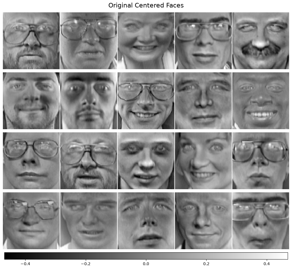
In this example, we reconstruct facial images from a low-dimensional representation. The Olivetti faces dataset contains 400 photos of 40 people, each of 64 × 64 = 4,096 pixels. Each photo is a sample and each pixel a variable. PCA needs every pixel to have mean zero across the photos. scikit-learn’s PCA subtracts these means itself, so the explicit global centering in the code is not needed for the PCA, but it makes the plotted faces show deviations from the average face. The local centering subtracts each photo’s own mean, which removes differences in overall brightness between the photos.
The principal components of this dataset are called eigenfaces. Each eigenface is a pattern over all 4,096 pixels that captures a direction of large variation between the faces (e.g., eyes, nose, or general facial structure). An eigenface plays the role of the gene-specific vector : it holds one value per pixel. The matching photo-specific scores play the role of the sample-specific vector : they say how much of each eigenface is present in each photo.
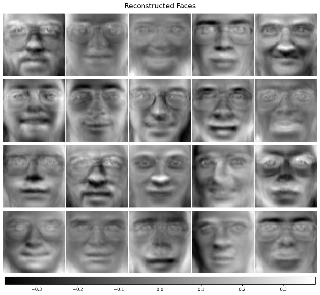
Projecting a face onto the 20 eigenfaces turns its 4,096 pixel values into 20 scores. The reconstruction (inverse_transform) reverses the process by adding up the eigenfaces, weighted by the face’s scores. The reconstructed faces are blurred but still recognizable, although each of them is described by 20 numbers instead of 4,096. The last plot shows why they are not perfect: the first eigenface explains 18% of the variance and the 20 eigenfaces together about 70%, so the remaining 30% of the variation, the finer detail, is lost.
What you should know after reading this chapter
You should be able to:
Calculate the outer product of two small vectors by hand, and explain how PCA does the reverse by finding the vectors and for which .
Interpret as gene-specific effects and as sample-specific effects of a genes samples matrix. Explain that is, up to a scaling factor, the projection of on , and vice versa.
Explain why the magnitude of a component can be moved freely between and , and how scaling both to unit length, , puts the whole magnitude in the singular value .
Describe how the second and later principal components are found by decomposing the residual , and state how many components a matrix can have at most.
Explain why the data are centered before PCA. Write down the singular value decomposition , and identify which matrix holds the gene-specific effects, the sample-specific effects and the singular values. Calculate the fraction of variance explained by component , , from a set of singular values.
Explain how PCA reduces the dimensionality of data, and interpret a scree plot of the explained variance per component to judge how many components to keep.
Explain how a sample is reconstructed approximately as a weighted sum of a few principal components, as when the eigenfaces example represents each 4,096-pixel face by only 20 numbers.