Differential expression analysis of two inbred mouse strains

Most RNA-seq experiments you will meet in the literature compare three samples against three samples. That is too few replicates to see what a $p$ value distribution actually looks like. We will therefore work with a more generously replicated data set: the mouse RNA-seq experiment of Bottomly et al. (2011), which compares gene expression in the striatum, a region of the brain, between two inbred mouse strains, 10 C57BL/6J mice and 11 DBA/2J mice, all of them adult males.

C57BL/6J (abbreviated B6) and DBA/2J (D2) are two of the most widely used laboratory mouse strains. B6 is the strain the mouse reference genome was sequenced from, and the two strains have been extensively characterised for behavioural and other striatum-related traits. Genetically they differ at millions of positions in their genomes. Within a strain, on the other hand, the mice are inbred and therefore genetically almost identical. The variation between the replicates of one strain is consequently not genetic, but stems from everything else that differs between two animals and two sequencing libraries.

The data set has since been reused in several comparisons of differential expression methods. We use the gene count table prepared by the ReCount project, which holds one read count per gene and sample, together with a table describing the samples. Both are downloaded once and cached. (The raw reads are available from the Sequence Read Archive under accession SRA026846.)

The rows of mouse are the genes, named by their Ensembl identifiers, and the columns are the 21 samples, named by their accession numbers in the Sequence Read Archive.

Before any further analysis we clean our data. Most of the 36,536 genes in the table are not expressed in the striatum, or only at a level where a handful of reads decide the outcome. We keep the genes with at least 10 reads in every sample.

Sequencing libraries differ in depth, so a raw count is not comparable between samples. We divide each sample by a size factor, the median over all genes of the ratio between the sample’s count and the gene’s geometric mean count across all samples, and then log transform. It is generally assumed that expression values follow a log-normal distribution, and hence the log transformation implies that the new values follow a normal distribution.

We can get an overview of the expression data:

and of the samples themselves, i.e. which strain each sample belongs to, on which of the three sequencing flow cells (experiment) it was sequenced, how deeply it was sequenced, and the size factor we just estimated for it:

Differential expression analysis¶

The goal of the exercise is to determine which genes are differentially expressed in the striatum of D2 mice as compared to B6 mice.

We first create a vector of booleans that tracks which samples are from D2 mice. This will be needed as an input for subsequent significance estimation.

Next, for each gene that has been measured, we calculate (1) the log fold change between the two strains, i.e. the difference between the mean log$_2$ expression values of the two strains, and (2) the significance of the difference between the strains.

An easy way to do so is by defining a separate function, get_significance_two_groups(row), that can do such calculations for any row of the expr DataFrame, and subsequently we use the function apply for the function to execute on each row of the DataFrame. For the significance test we use a $t$ test, which is provided by the function ttest_ind. With equal_var=False it performs Welch’s $t$ test, which, unlike the pooled $t$ test of the previous chapter, does not assume that the expression of a gene varies equally much in the two strains.

This results in a new table with gene names, their $p$ values of differential expression, and their log fold changes.

A common way to illustrate the differential expression values is to plot the negative log of the $p$ values as a function of the $\log_2$ fold change of each gene. This is known as a Volcano plot.

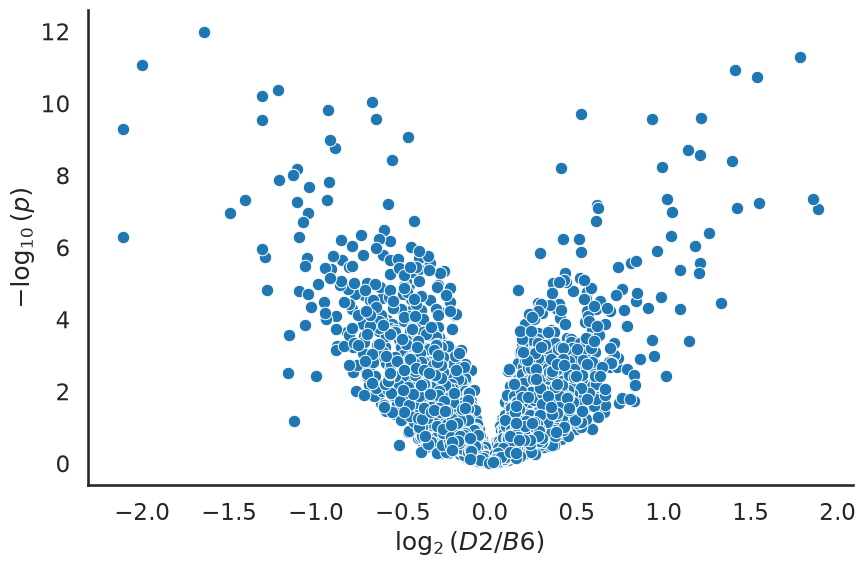
The genes in the top left and top right corners are the most interesting ones, as they combine a large fold change with a small $p$ value.

We can count how many genes we would call significant at the conventional threshold $p<0.05$, and compare that to the number we would expect to see by pure chance if no gene at all were differentially expressed.

How much does the number of replicates matter?¶

The analysis above used all 21 samples, which is more than most experiments can afford. With this data set we can pretend to have run a smaller experiment, simply by drawing a subset of the replicates, and see what we would have concluded.

Below we draw $n$ B6 and $n$ D2 replicates at random, repeat the whole $t$ test for every gene, and record how many genes pass $p<0.05$. To keep the repeated analysis fast we use a vectorised version of the same Welch $t$ test as above, testing all genes in one call.

The $p$ value histograms tell the same story in a more informative way. For each $n$ we show the draw whose number of genes below $p<0.05$ is closest to the median of the 20 draws. A histogram of $p$ values is a mixture of a flat, uniform part, stemming from the genes that follow the null hypothesis $H_0$, and a spike close to zero, stemming from the genes that are truly differentially expressed. The dashed line marks the height the histogram would have if every gene followed $H_0$.

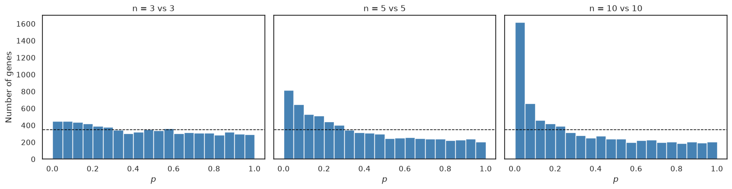
Two things are worth noticing. First, the spike at low $p$ grows steadily with the number of replicates, and at three versus three it is barely visible. The genes are just as differentially expressed in the small experiment as in the large one; we are simply unable to demonstrate it. Here, statistical power is bought with replicates. Sequencing the same mice more deeply would reduce the counting noise, which mainly matters for lowly expressed genes, but not the variation between animals. Second, the result of a three-versus-three experiment is unstable — the lowest and highest columns of the table above show how much the number of findings varies between two equally valid draws of three replicates per strain.

This is also a warning about how to read the literature. A gene that appears in a three-versus-three study and not in another is not necessarily a contradiction; it may simply be two draws from the same lottery.

Finally, note that the flat part of the histograms, from the genes that follow $H_0$, extends all the way down to $p=0$, so some of the genes below $p<0.05$ are not differentially expressed. If all $m$ tested genes were null, we would expect $0.05m$ false positives at that threshold, regardless of the number of replicates. As some of the genes are truly differentially expressed, $0.05m$ is an upper bound on the expected number of false positives. How to deal with that problem is the topic of the next chapter.