q value calculations in a comparison of two mouse strains

Differential expression analysis with multiple testing¶

This chapter applies the methods of the previous chapter to the analysis of the chapter on differential expression in two mouse strains.

We again compare the striatum of the two inbred mouse strains C57BL/6J (B6, 10 mice) and DBA/2J (D2, 11 mice), from the RNA-seq experiment of Bottomly et al. (2011), using the gene count table prepared by the ReCount project.

We first recreate the steps of that chapter. Since we will repeat the testing several times in this chapter, we write the $t$ test in a vectorised form that tests all genes in a single call, rather than looping over the rows of the table.

# When the page runs in the browser (JupyterLite), we install seaborn, and fetch the data from a copy in the book's
# repository, as the ReCount server does not allow downloads from within a browser
import sys
if sys.platform == "emscripten":
    import os
    import micropip
    await micropip.install(["seaborn", "pyodide-http"])
    import pyodide_http
    pyodide_http.patch_all()
    from urllib.request import urlretrieve
    repo = "https://raw.githubusercontent.com/statisticalbiotechnology/dsbook/main/dsbook/statistics/data/"
    data_dir = "../data" if os.path.isdir("../data") else "data"
    os.makedirs(data_dir, exist_ok=True)
    for file_name in ["bottomly_count_table.txt", "bottomly_phenodata.txt"]:
        if not os.path.exists(os.path.join(data_dir, file_name)):
            urlretrieve(repo + file_name, os.path.join(data_dir, file_name))

import os
import urllib.request

import numpy as np
import pandas as pd
from scipy.stats import ttest_ind

data_dir = "../data" if os.path.isdir("../data") else "data"
os.makedirs(data_dir, exist_ok=True)

recount_url = "https://bowtie-bio.sourceforge.net/recount/"
for folder, file_name in [("countTables/", "bottomly_count_table.txt"),
                          ("phenotypeTables/", "bottomly_phenodata.txt")]:
    local_file = os.path.join(data_dir, file_name)
    if not os.path.exists(local_file):
        urllib.request.urlretrieve(recount_url + folder + file_name, local_file)

mouse = pd.read_csv(os.path.join(data_dir, "bottomly_count_table.txt"), sep="\t", index_col=0)
pheno = pd.read_csv(os.path.join(data_dir, "bottomly_phenodata.txt"), sep=" ", index_col=0)

mouse = mouse.loc[(mouse >= 10).all(axis=1)]
log_counts = np.log(mouse)
size_factors = np.exp(log_counts.sub(log_counts.mean(axis=1), axis=0).median(axis=0))
expr = np.log2(mouse.div(size_factors, axis=1))

strain = pheno.loc[expr.columns, "strain"]
b6_samples = list(expr.columns[strain == "C57BL/6J"])
d2_samples = list(expr.columns[strain == "DBA/2J"])

def get_significance_two_groups(data, group_a, group_b):
    "Welch t test of every gene, comparing the samples of group_a to those of group_b."
    log_fold_change = data[group_a].mean(axis=1) - data[group_b].mean(axis=1)
    p = ttest_ind(data[group_a], data[group_b], axis=1, equal_var=False)[1]
    return pd.DataFrame({"p": p, "-log_p": -np.log10(p), "log_FC": log_fold_change.values},
                        index=data.index)

pvalues = get_significance_two_groups(expr, d2_samples, b6_samples)

When plotting the $p$ value distribution below, we see an enrichment of low $p$ values. Most of these come from genes that follow the alternative hypothesis. We also see a uniform distribution of the $p$ values in the higher end of the distribution, i.e. $p$ values of 0.5–1.0. These are likely stemming from genes that follow $H_0$ .

import seaborn as sns
import matplotlib.pyplot as plt
plt.figure(figsize=(12, 8))
sns.histplot(x=pvalues["p"],kde=False)
plt.xlim(0,1.0);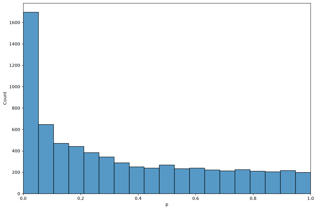

$q$ value estimation¶

We define a function for the calculation of $\pi_0$ . Here we use a different method than the spline described by Storey & Tibshirani, namely the bootstrap method of Storey (2002), which is outlined in a note in the previous chapter. As the method is based on random resampling, we fix the seed of the random number generator, so that the estimate is the same every time we run the analysis.

def estimatePi0(p, numBoot=100, numLambda=100, maxLambda=0.95, seed=0):
    "Bootstrap estimate of pi_0, the fraction of p values that stem from true null hypotheses."
    rng = np.random.default_rng(seed)
    p = np.asarray(p)
    n = len(p)
    lambdas = np.linspace(maxLambda/numLambda, maxLambda, numLambda)
    # pi_0(lambda) = |{p_i > lambda}| / (n (1 - lambda)) for each lambda
    pi0s = np.array([(p > l).sum() / (n * (1 - l)) for l in lambdas])
    minPi0 = np.min(pi0s)
    mse = np.zeros(numLambda)
    for boot in range(numBoot):
        pBoot = rng.choice(p, n, replace=True)   # resample the p values with replacement
        pi0sBoot = np.array([(pBoot > l).sum() / (n * (1 - l)) for l in lambdas])
        mse = mse + np.square(pi0sBoot - minPi0)
    return pi0s[np.argmin(mse)]

Following Storey & Tibshirani, we first calculate

\hat{\rm FDR}(t) = \frac{\hat{\pi}_0 m t}{|\{p_i\le t\}|},

(1)

and then make the $\hat{\rm FDR}(t)$ estimates monotone by taking the minimum over all thresholds at least as large as $p_i$ ,

\hat{q}(p_i)=\min_{t \ge p_i}\hat{\rm FDR}(t).

(2)

def qvalues(pvalues):
    "Return a copy of the table, sorted in ascending order of p value, with an added column of q values."
    qv = pvalues.sort_values("p")   # a sorted copy; the input table is left unchanged
    m = qv.shape[0]                 # the number of p values
    p = qv["p"].values
    pi0 = estimatePi0(p)
    print(f"pi_0 estimated to {pi0:.3f}")

    # calculate FDR(t) at each threshold t = p_(i), as in Storey & Tibshirani
    fdr = [pi0 * p[i] * m / (i + 1) for i in range(m)]

    # calculate q(p_i) as the minimal FDR(t) over all t >= p_i, walking from the largest p value down
    q = np.zeros(m)
    old_q = 1.0
    for i in reversed(range(m)):
        old_q = min(old_q, fdr[i])
        q[i] = old_q
    qv["q"] = q
    return qv

qv = qvalues(pvalues)

pi_0 estimated to 0.544

The estimated $\pi_0$ of about 0.5 says that roughly half of the expressed genes differ in their expression between the two strains. Given that the strains differ at millions of positions in their genomes, many of them in sequences that regulate gene expression, that is not unreasonable. One might worry that some of the differences are technical: the reads were aligned to the reference genome, which is a B6 genome, so reads from D2 genes carrying many sequence differences could align less well and make those genes look lower expressed in D2. Bottomly et al. tested this by realigning the D2 reads to a D2 version of the genome, and found that the effect on their results was minimal.

Note that $\pi_0$ and the $q$ values answer different questions. $\pi_0$ estimates how many genes are differentially expressed in total, while a $q$ value tells us which genes we can single out with a controlled error rate. Many of the expression differences are too small to be pinned down gene by gene with ten mice per strain, even though their combined effect on the $p$ value distribution is clearly visible. (Bottomly et al. used a test designed for count data, and reported 1,727 differentially expressed genes at $q<0.01$ out of the 16,183 genes they tested.)

The table lists the genes in descending order of significance, together with their $q$ values.

qv

Displaying number of findings as a function of $q$ value¶

A plot of the number of differentially expressed genes as a function of the $q$ value threshold shows how many genes we can report at each FDR level.

plt.plot(qv["q"], np.arange(1, qv.shape[0] + 1), lw=3)
plt.xlim(0, 0.1)
plt.ylim(0, (qv["q"] < 0.1).sum())
plt.xlabel("$q$ value threshold")
plt.ylabel("Number of differential genes");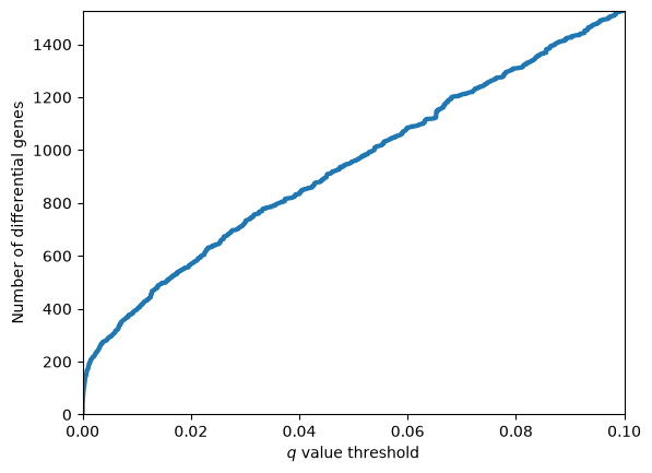

Volcano plots revisited¶

We often see that Volcano plots are complemented with FDR thresholds. Here we complement the volcano plot of the mouse strain chapter with coloring indicating if genes are significantly differentially expressed at an FDR threshold of 0.01.

qv["Significant"] = qv["q"]<0.01
less_than_FDR_1 = qv[qv["q"]<0.01]
p_threshold = less_than_FDR_1.iloc[-1]["-log_p"]
print(f"{len(less_than_FDR_1)} of {len(qv)} genes have q < 0.01")

395 of 6995 genes have q < 0.01

import matplotlib.pyplot as plt
import seaborn as sns

sns.set_style("white")
sns.set_context("talk")
ax = sns.relplot(data=qv,x="log_FC",y="-log_p",hue="Significant",aspect=1.5,height=6)
plt.axhline(p_threshold)
ax.set(xlabel=r"$\log_2(D2/B6)$", ylabel=r"$-\log_{10}(p)$");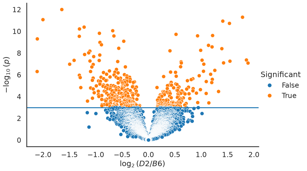

A ground truth null experiment¶

A $p$ value histogram that is enriched near zero, and a $\pi_0$ well below one, are easy to produce. The harder question is whether we should believe them: how do we know that the machinery above is not manufacturing findings out of technical artefacts?

Most data sets cannot answer that question, because we never know which genes are truly differentially expressed. This data set lets us construct such a case. The ten B6 mice are inbred, i.e. genetically almost identical, and were all treated the same way. If we split them into two groups of five, we have built an experiment in which the null hypothesis is true for every single gene. Any finding is by construction a false positive.

The B6 mice were sequenced on three different flow cells (the experiment column of the sample table in the mouse strain chapter). To keep the comparison fair, we alternate the mice of each flow cell between the two groups, so that both groups contain mice from all three flow cells.

sns.set_context("notebook")
flow_cell = pheno["experiment.number"]
b6_by_flow_cell = sorted(b6_samples, key=lambda s: flow_cell[s])
group_a, group_b = b6_by_flow_cell[0::2], b6_by_flow_cell[1::2]

null_pvalues = get_significance_two_groups(expr, group_a, group_b)

m = null_pvalues.shape[0]
bins = 20
fig, ax = plt.subplots(1, 2, figsize=(13, 4.5), sharey=False)
ax[0].hist(null_pvalues["p"], bins=bins, range=(0, 1), color="steelblue")
ax[0].axhline(m / bins, color="k", ls="--", lw=1)
ax[0].set_title("B6 vs B6, 5 vs 5 (all $H_0$)")
ax[1].hist(qv["p"], bins=bins, range=(0, 1), color="indianred")
ax[1].axhline(m / bins, color="k", ls="--", lw=1)
ax[1].set_title("D2 vs B6, 11 vs 10")
for a in ax:
    a.set_xlabel("$p$"); a.set_ylabel("Number of genes")
plt.tight_layout();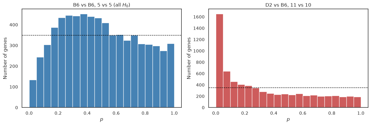

The difference is striking. The B6 against B6 comparison has no spike at all near zero, so the test does not manufacture findings out of nothing. The histogram is, however, not perfectly flat either: small $p$ values are rarer than the uniform distribution predicts (the dashed line marks the height $m/20$ of a uniform distribution), and intermediate ones more common. The reason is the flow cells. Each of our two groups contains mice from all three flow cells, so the differences between flow cells inflate the variance within each group, while they largely cancel out in the difference between the group means (the split is 2/2/1 against 1/2/2 mice from the three flow cells, so the cancellation is not perfect). The $t$ statistics therefore come out smaller than they should, and the $p$ values larger. In other words, the test becomes conservative. The same applies to the comparison between the strains, as Bottomly et al. spread the mice of both strains over all three flow cells, so we lose some power there too.

Running the same $q$ value machinery on this null experiment should therefore report no findings.

null_qv = qvalues(null_pvalues)
for threshold in (0.01, 0.05, 0.10, 0.20):
    print(f"genes with q < {threshold:4.2f}: {int((null_qv['q'] < threshold).sum()):5d}"
          f"   (out of {m})")
print("smallest q value in the null experiment: %.3f" % null_qv["q"].min())

pi_0 estimated to 0.848
genes with q < 0.01:     0   (out of 6995)
genes with q < 0.05:     0   (out of 6995)
genes with q < 0.10:     0   (out of 6995)
genes with q < 0.20:     0   (out of 6995)
smallest q value in the null experiment: 0.789

No gene survives any reasonable $q$ value threshold, whereas the real comparison produced hundreds of findings at $q<0.01$ . The multiple hypothesis correction is not simply throwing away everything, nor is it rubber-stamping noise. Note, though, that the estimated $\pi_0$ comes out below one, as the estimate assumes that the true nulls give a flat histogram, which they do not quite do here.

A batch effect¶

The care we took to balance the flow cells was not a formality. Below we instead compare the four B6 mice sequenced on flow cell 6 to the six sequenced on flow cells 4 and 7. The null hypothesis is still true for every gene in a biological sense, as all ten mice are B6, but now the two groups also differ in how they were processed.

batch_a = [s for s in b6_samples if flow_cell[s] == 6]
batch_b = [s for s in b6_samples if flow_cell[s] != 6]
batch_pvalues = get_significance_two_groups(expr, batch_a, batch_b)

plt.figure(figsize=(6.5, 4.5))
plt.hist(batch_pvalues["p"], bins=bins, range=(0, 1), color="darkorange")
plt.axhline(m / bins, color="k", ls="--", lw=1)
plt.title("B6 flow cell 6 vs B6 flow cells 4 and 7")
plt.xlabel("$p$"); plt.ylabel("Number of genes");
batch_qv = qvalues(batch_pvalues)
print(f"genes with q < 0.05: {int((batch_qv['q'] < 0.05).sum())}")

pi_0 estimated to 0.553
genes with q < 0.05: 3

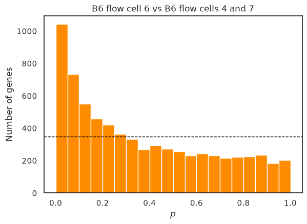
Now the histogram shows a clear spike of small $p$ values, $\pi_0$ is estimated well below one, and the $q$ value machinery even reports a few significant genes, although none of them is differentially expressed in a biological sense. The $t$ test cannot tell a difference caused by biology from a difference caused by the processing of the samples. Batch effects thus cut both ways: when the batches are confounded with the groups they create false findings, and when they are spread over the groups they inflate the variance and cost power, as we saw above. This is why a good experimental design spreads the conditions evenly over the processing batches, as Bottomly et al. did for the two strains, and why more advanced analyses include the batch as an explanatory variable in the model, rather than leaving it in the noise.

Spline estimation of $\pi_0$ ¶

Storey and Tibshirani estimate $\pi_0$ differently from the bootstrap procedure used above: they compute $\hat{\pi}_0(\lambda) = \frac{|\{p_i>\lambda \}|}{m(1-\lambda)}$ for a range of $\lambda$ values and smooth these estimates with a spline.

Below, we almost follow the article’s described procedure (please try to find the difference in how we select which lambdas we evaluate). We fit a smoothing cubic spline to the $\hat{\pi}_0(\lambda)$ estimates.

from scipy.interpolate import UnivariateSpline

lambdas = qv["p"].values                 # the p values, sorted in ascending order
m = len(lambdas)                         # the number of p values
num_above = m - 1 - np.arange(m)         # the number of p values greater than each lambda
pi0_hat = num_above / (m * (1 - lambdas))

s = UnivariateSpline(lambdas, pi0_hat, k=3, s=10)

We plot the estimates (blue) as well as the spline fit (red) for two different intervals of $\lambda$ . You will see the need for a smoother, particularly in the region near 1.0.

def plot_pi0_hat(lambdas, pi0_hat, s, xlow, xhigh, ax):
    ax.plot(lambdas, pi0_hat, lw=3, color='b')
    ax.plot(lambdas, s(lambdas), lw=3, color='r')
    ax.set_xlim(xlow, xhigh)
    ax.set_ylim(0, 1.05)
    ax.set_xlabel(r"$\lambda$")
    ax.set_ylabel(r"$\hat{\pi}_0(\lambda)$")

fig, ax = plt.subplots(1, 2, figsize=(12, 4))
plot_pi0_hat(lambdas, pi0_hat, s, 0, 1, ax[0])
plot_pi0_hat(lambdas, pi0_hat, s, 0.95, 1, ax[1])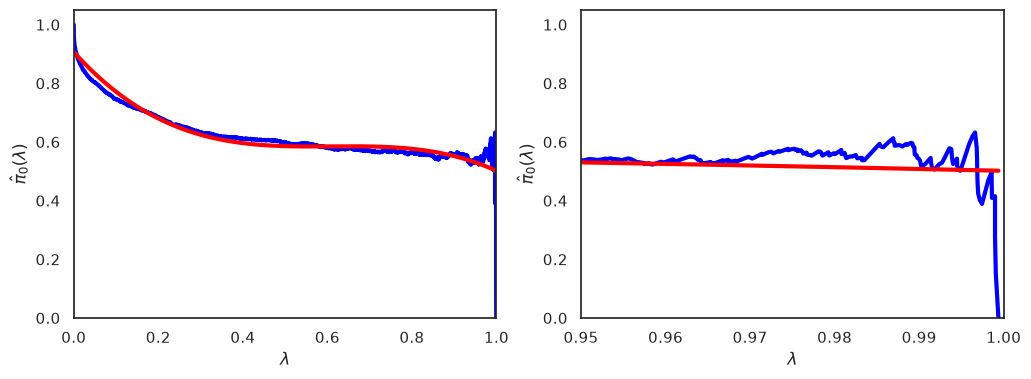

We can obtain a final estimate by evaluating the spline for $\lambda=1$ , and compare it to the bootstrapping estimate.

print(f"Spline estimate of pi_0:    {float(s(1)):.3f}")
print(f"Bootstrap estimate of pi_0: {estimatePi0(qv['p'].values):.3f}")

Spline estimate of pi_0:    0.502
Bootstrap estimate of pi_0: 0.544

References¶

Bottomly, D., Walter, N. A. R., Hunter, J. E., Darakjian, P., Kawane, S., Buck, K. J., Searles, R. P., Mooney, M., McWeeney, S. K., & Hitzemann, R. (2011). Evaluating Gene Expression in C57BL/6J and DBA/2J Mouse Striatum Using RNA-Seq and Microarrays. PLoS ONE, 6(3), e17820. 10.1371/journal.pone.0017820
Frazee, A. C., Langmead, B., & Leek, J. T. (2011). ReCount: A multi-experiment resource of analysis-ready RNA-seq gene count datasets. BMC Bioinformatics, 12(1). 10.1186/1471-2105-12-449
Storey, J. D. (2002). A Direct Approach to False Discovery Rates. Journal of the Royal Statistical Society Series B: Statistical Methodology, 64(3), 479–498. 10.1111/1467-9868.00346