Hypothesis Testing

Hypothesis testing is a statistical procedure used to determine if a sample data set provides sufficient evidence to reject a stated null hypothesis ($H_0$) in favor of an alternative hypothesis ($H_1$). This method is fundamental in science for drawing inferences about populations based on sample data. It allows researchers to judge whether their observations could plausibly have arisen by chance alone, if there were no genuine effect.

Statistical hypothesis test¶

Null Hypothesis ($H_0$) and Alternative Hypothesis ($H_1$)¶

In hypothesis testing, we begin by stating two competing hypotheses about a population or a set of populations:

• Null Hypothesis ($H_0$): This is a statement suggesting there is no effect, relationship, or difference. It represents the status quo or a baseline assumption. For example, in a clinical trial, $H_0$ might state that a new drug has no effect compared to a placebo (i.e. patients in the placebo population do not differ from those in the population of treated patients).

• Alternative Hypothesis ($H_1$): This hypothesis reflects what the researcher aims to prove. It suggests that there is an effect, a relationship, or a difference. In the clinical trial example, $H_1$ would state that the new drug has a beneficial effect compared to the placebo.

The purpose of hypothesis testing is to assess whether the data provides enough evidence to reject $H_0$ in favor of $H_1$. This process involves comparing the observed data in a sample to what we would expect under $H_0$.

Test Statistics¶

A test statistic is a value calculated from sample data that allows us to make a decision about the hypotheses. One commonly used test statistic is the difference in means between two samples. For example, if we want to compare the average effect of a treatment versus a placebo, we calculate the difference in the sample means for the two groups. The test statistic helps determine how far the observed data deviates from what we would expect under $H_0$, which typically assumes that there is no difference in means between the groups.

Sampling Distribution under the Null Hypothesis¶

The sampling distribution under the null hypothesis is the distribution of the test statistic assuming that $H_0$ is true. This distribution helps us understand the range of possible values the test statistic can take if the null hypothesis is correct. By comparing the observed test statistic to this distribution, we can determine how likely it is to observe such a value by random chance alone. This comparison is essential for calculating the $p$ value.

$p$ value¶

The $p$ value represents the probability of obtaining the observed data, or something more extreme, if the null hypothesis were true. It is used as a measure of evidence against $H_0$:

• A smaller $p$ value suggests that the observed data would be unlikely under $H_0$, providing stronger evidence against the null hypothesis.

• For example, a $p$ value of 0.03 means there is a 3% chance of observing the data (or something more extreme) if $H_0$ is true, which would lead us to consider rejecting $H_0$.

Significance Level ($\alpha$)¶

The significance level (denoted as $\alpha$) is a predetermined threshold that determines whether the $p$ value is considered small enough to reject the null hypothesis. A common choice for $\alpha$ is 0.05, which means we are willing to accept a 5% chance of incorrectly rejecting $H_0$ (Type I error):

• If the $p$ value is less than $\alpha$, the results are considered statistically significant, and we reject $H_0$.

• The choice of $\alpha$ depends on the context of the study and the consequences of making an error. For example, in medical research, a smaller $\alpha$ (e.g., 0.01) might be chosen to reduce the risk of false positives.

False Positives and False Negatives¶

In hypothesis testing, two types of errors can occur:

• False Positive (Type I Error): Rejecting $H_0$ when it is actually true. This error can lead to incorrect conclusions, such as believing a treatment is effective when it is not.

• False Negative (Type II Error): Failing to reject $H_0$ when the alternative hypothesis is true. This error can result in missed discoveries, such as failing to detect a real effect or relationship.

The two types of error trade off against each other: lowering $\alpha$ reduces the risk of false positives, but makes it harder to detect real effects, and so increases the risk of false negatives.

Limitations & Misinterpretations¶

While hypothesis testing is powerful, it has its limitations and can be easily misinterpreted:

• A $p$ value measures the strength of evidence against $H_0$, not the size of the effect. With enough data, a medical treatment can show a statistically significant improvement that is too small to be of any practical significance to patients, and a large effect can fail to reach significance in a small study. Results must therefore be interpreted in the context of the research question.

• A $p$ value does not give the probability that either hypothesis is true. It only tells us how compatible the observed data are with $H_0$.

Assessing Significance Using Permutation Testing¶

We can use permutation testing to evaluate significance. The null hypothesis is that there is no relationship between the measured values and the labels attached to them, such as between a measurement and the group of the sample it was made on, or between the dependent variable $y$ and the independent variable $\mathbf{x}$ of a regression. If so, any random pairing of values and labels is as likely as the observed one. Shuffling the labels many times, and recalculating the test statistic each time, therefore gives us the null distribution of the test statistic, to which we compare the observed value to compute a $p$ value.

Why Permutation Testing?¶

Permutation testing is non-parametric, meaning it doesn’t assume a specific distribution of the residuals or the coefficients. This makes it a powerful and flexible method, especially in cases where the assumptions of parametric tests (e.g., normality) might not hold. Further, we here use it as a pedagogic tool, to understand how frequentist hypothesis testing actually works.

Step-by-step Procedure¶

1. Calculate the test statistic on the original data, e.g. the difference in means between two groups, or the loss of a model fitted to the data.

2. Permute the labels (shuffle the group labels, or shuffle $y$ while keeping $\mathbf{x}$ unchanged) and recalculate the test statistic on the permuted data, refitting the model if there is one.

3. Repeat the permutation process many times to build a distribution of the test statistic under the null hypothesis.

4. Calculate the $p$ value as the fraction of permuted test statistics that are at least as extreme as the observed one.

Permutation Test for Comparing the Means of Two Samples¶

We first test whether two samples have different means. Here we shuffle the group labels, and use the absolute difference between the two sample means as test statistic. As a large difference in either direction counts as extreme, this is a two-sided test (see below).

# When the page runs in the browser (JupyterLite), seaborn is not preinstalled, so we install it first
import sys
if sys.platform == "emscripten":
    import micropip
    await micropip.install("seaborn")

import numpy as np
import seaborn as sns
import matplotlib.pyplot as plt

# Generate two normally distributed samples with slightly different means
rng = np.random.RandomState(2)
sample1 = rng.normal(loc=0.0, scale=1.0, size=10)
sample2 = rng.normal(loc=0.4, scale=1.0, size=10)

# Plot the samples using swarmplot
data = {'value': np.concatenate([sample1, sample2]),
        'group': ['Sample 1'] * len(sample1) + ['Sample 2'] * len(sample2)}

sns.swarmplot(x='group', y='value', data=data)
plt.show()

# Permutation test for difference in means
n_permutations = 1000
observed_diff = np.abs(np.mean(sample1) - np.mean(sample2))

combined = np.concatenate([sample1, sample2])
permuted_diffs = []

for _ in range(n_permutations):
    permuted = rng.permutation(combined)
    perm_sample1 = permuted[:len(sample1)]
    perm_sample2 = permuted[len(sample1):]
    permuted_diff = np.abs(np.mean(perm_sample1) - np.mean(perm_sample2))
    permuted_diffs.append(permuted_diff)

# Compute the p-value by comparing the observed difference to the null distribution
permuted_diffs = np.array(permuted_diffs)
p_value = np.mean(permuted_diffs >= observed_diff)

# Plot the null distribution and observed difference
plt.hist(permuted_diffs, bins=30, alpha=0.7, label="Permuted Differences")
plt.axvline(observed_diff, color='r', linestyle='--', label=f"Observed Diff = {observed_diff:.2f}")
plt.title(f"Permutation Test for Difference in Means (p value = {p_value:.4f})")
plt.xlabel("Absolute Difference in Means")
plt.ylabel("Frequency")
plt.legend()
plt.show()

print(f"Observed difference in means: {observed_diff:.4f}")
print(f"p value from permutation test: {p_value:.4f}")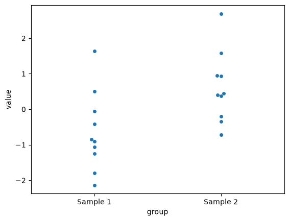

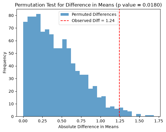
Observed difference in means: 1.2441
p value from permutation test: 0.0180

Permutation Test for Model Significance¶

Next, we test whether a linear regression model explains any of the variation in $y$, using the model’s SSE as test statistic. Here a small loss is extreme, so the $p$ value is the fraction of permuted losses that are at most as large as the observed loss.

import numpy as np
from scipy.optimize import minimize
import seaborn as sns
import matplotlib.pyplot as plt

# Generate synthetic data
rng = np.random.RandomState(42)
x = rng.rand(50)
y = 1.2 * x - 0.5 + 1.1 * rng.randn(50)

# Define the linear model
def linear_model(params, x):
    slope, intercept = params
    return slope * x + intercept

# Define the loss function (sum of squared residuals)
def loss(params, x, y):
    return np.sum((y - linear_model(params, x))**2)

# Fit the model to the original data
initial_params = rng.randn(2)
result = minimize(loss, initial_params, args=(x, y))
observed_loss = result.fun

# Permutation test
n_permutations = 1000
permuted_losses = []

for _ in range(n_permutations):
    # Shuffle y and fit the model to the permuted data
    y_permuted = rng.permutation(y)
    permuted_result = minimize(loss, initial_params, args=(x, y_permuted))
    permuted_losses.append(permuted_result.fun)

# Compute the p-value by comparing the observed loss to the null distribution
permuted_losses = np.array(permuted_losses)
p_value = np.mean(permuted_losses <= observed_loss)

# Plot the null distribution and observed loss
plt.hist(permuted_losses, bins=30, alpha=0.7, label="Permuted Losses")
plt.axvline(observed_loss, color='r', linestyle='--', label=f"Observed Loss = {observed_loss:.2f}")
plt.title(f"Permutation Test for Model Significance (p value = {p_value:.4f})")
plt.xlabel("SSE Loss")
plt.ylabel("Frequency")
plt.legend()
plt.show()

print(f"Observed loss: {observed_loss:.4f}")
print(f"p value from permutation test: {p_value:.4f}")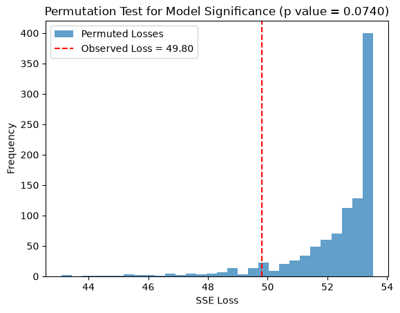

Observed loss: 49.7958
p value from permutation test: 0.0740

t-tests¶

When the population from which your samples are drawn is normally distributed, a t-test can be used to evaluate whether there is a significant difference between the means of two independent groups. Under these conditions the difference in sample means is normally distributed, and dividing it by its estimated standard error yields a t-statistic, which follows a t-distribution. It is the extra uncertainty from estimating the standard deviation from the data, rather than knowing it, that gives the t-distribution its heavier tails. This allows us to calculate the probability ($p$ value) of observing a difference as large as (or larger than) the one obtained, assuming the null hypothesis is true.

Below we use SciPy’s ttest_ind, which by default performs Student’s $t$-test. Student’s test also assumes that the two groups have the same variance; with the argument equal_var=False, ttest_ind instead performs Welch’s $t$-test, which does not.

import numpy as np
from scipy.stats import ttest_ind

# Perform a two-sample t-test (on the same two samples as in the first permutation test)
t_stat, p_value = ttest_ind(sample1, sample2)

print(f"p value: {p_value:.4f}")

p value: 0.0168

When the data really are normally distributed, the $t$-test is the most powerful test of a difference in means, i.e. the one most likely to detect a real difference. A permutation test on the same data is usually almost as powerful; for our two samples, the $t$-test gives $p = 0.017$ and the permutation test $p = 0.018$. The advantage of the $t$-test shows up for very small samples. A permutation test can only produce as many distinct $p$ values as there are distinct ways to permute the labels, e.g. $\binom{6}{3} = 20$ for three against three samples, so its smallest possible two-sided $p$ value is then $2/20 = 0.1$, whereas a $t$-test can produce arbitrarily small $p$ values. In return, the $t$-test’s $p$ values are only accurate if the normality assumption holds, which is hard to check in small samples, while the permutation test makes no such assumption.

One- vs Two-sided tests¶

A one-sided test is used when we want to determine if there is a difference in a specific direction (e.g., whether one group mean is greater than the other). In contrast, a two-sided test checks if there is any difference between the groups, regardless of direction (i.e., whether one mean is greater or less than the other). A two-sided test is more conservative because it tests for deviations in both directions, while a one-sided test focuses on a predetermined outcome.

Below, we repeat the permutation test on the same two samples as before, but now test one-sidedly whether sample2 has a larger mean than sample1. The test statistic is $\Delta = \bar{x}_2 - \bar{x}_1$, the mean of sample2 minus the mean of sample1, without taking absolute values:

import numpy as np
import matplotlib.pyplot as plt
from IPython.display import display, Markdown, Math

rng = np.random.RandomState(0)

# One-sided permutation test for difference in means (Sample 2 > Sample 1)
n_permutations = 1000
observed_diff = np.mean(sample2) - np.mean(sample1)

combined = np.concatenate([sample1, sample2])
permuted_diffs = []

for _ in range(n_permutations):
    permuted = rng.permutation(combined)
    perm_sample1 = permuted[:len(sample1)]
    perm_sample2 = permuted[len(sample1):]
    permuted_diff = np.mean(perm_sample2) - np.mean(perm_sample1)
    permuted_diffs.append(permuted_diff)

# Compute the one-sided p values for either direction, and the two-sided p value
permuted_diffs = np.array(permuted_diffs)
ge_p_value = np.mean(permuted_diffs >= observed_diff)
le_p_value = np.mean(permuted_diffs <= observed_diff)
two_p_value = np.mean(abs(permuted_diffs) >= abs(observed_diff))

# Plot the null distribution and observed difference
plt.hist(permuted_diffs, bins=30, alpha=0.7, label="Permuted Differences")
plt.axvline(observed_diff, color='r', linestyle='--', label=f"Observed Diff = {observed_diff:.2f}")
plt.xlabel("Difference in Means")
plt.ylabel("Frequency")
plt.legend()
plt.show()

display(Markdown(rf"Observed difference in means: {observed_diff:.4f}"))
display(Math(rf"p (H_0: \Delta \le 0): {ge_p_value:.4f}"))
display(Math(rf"p (H_0: \Delta \ge 0): {le_p_value:.4f}"))
display(Math(rf"p (H_0: \Delta = 0): {two_p_value:.4f}"))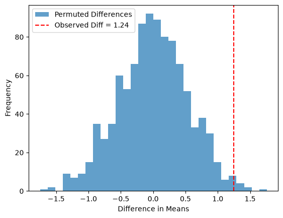

Loading...

Loading...

Loading...

Loading...

The one-sided test of $H_0: \Delta \le 0$ against $H_1: \Delta > 0$ uses only the right tail of the null distribution: its $p$ value is the fraction of permutations where perm_sample2 - perm_sample1 is at least as large as the observed difference. As the observed difference lies in the predicted direction, this $p$ value (0.009) is about half of the two-sided one (0.022), which counts extreme differences in both tails. Had we instead predicted that sample2 has the smaller mean, i.e. tested $H_0: \Delta \ge 0$, the $p$ value would have been close to 1. The direction of a one-sided test must therefore be decided before looking at the data; choosing it afterwards halves the $p$ value without justification.

When testing whether a drug is effective, the research question is directional, which can motivate a one-sided test. Note, however, that regulators of clinical trials usually require either a two-sided test at $\alpha = 0.05$ or a one-sided test at $\alpha = 0.025$, which amounts to the same evidence threshold, partly because a harmful effect of the drug is also important to detect. In differential gene expression analysis, you want to find both up- and downregulated genes, making a two-sided test the natural choice.

Power and sample size¶

The power of a test is the probability that it rejects $H_0$ when there really is a difference, i.e. the probability of avoiding a type II error. Power is a property of the experiment rather than of the data: it depends on how large the true difference is compared to the variation within the groups, on the number of samples per group, and on the significance level $\alpha$.

Before an experiment we cannot know the true difference, but we can decide on the smallest difference that would matter, and take an estimate of the variation from earlier data or a pilot experiment. With those two numbers we can run the experiment many times on the computer, analyze each simulated experiment just as we plan to analyze the real one, and count how often we reach $p < \alpha$. That fraction is the power.

To see the idea, we simulate 10,000 experiments with five samples per group, once in a world where $H_0$ is true and once in a world where the true means differ by one standard deviation (SD), and record the difference in means of each experiment:

import numpy as np
import matplotlib.pyplot as plt
from scipy import stats

rng = np.random.default_rng(0)
n, difference, n_experiments = 5, 1.0, 10000

# Difference in means of each simulated experiment, when H0 is true and when it is not
null_diffs = rng.normal(0, 1, (n_experiments, n)).mean(axis=1) - rng.normal(0, 1, (n_experiments, n)).mean(axis=1)
alt_diffs = rng.normal(difference, 1, (n_experiments, n)).mean(axis=1) - rng.normal(0, 1, (n_experiments, n)).mean(axis=1)

# Differences larger than 95% of the null differences give p < 0.05 (two-sided)
threshold = np.quantile(np.abs(null_diffs), 0.95)
power = np.mean(np.abs(alt_diffs) >= threshold)

bins = np.linspace(-3, 4, 71)
plt.hist(null_diffs, bins=bins, alpha=0.5, color="grey", label="$H_0$ true")
plt.hist(alt_diffs, bins=bins, alpha=0.5, color="tab:orange", label="True difference = 1 SD")
for x in (-threshold, threshold):
    plt.axvline(x, color="k", linestyle="--")
plt.xlabel("Difference in means")
plt.ylabel("Number of simulated experiments")
plt.legend()
plt.show()

print(f"Fraction of experiments with a significant difference: {power:.2f}")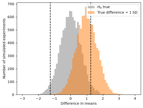

Fraction of experiments with a significant difference: 0.34

The grey histogram is the sampling distribution of the difference in means under $H_0$, and the dashed lines mark the differences that are extreme enough to give $p < 0.05$. The orange histogram shows what we would observe if the true difference were one SD. Only the experiments beyond the dashed lines give a significant result; with five samples per group that is about a third of them, so two experiments out of three would miss the difference.

To plan an experiment, we repeat the simulation for different numbers of samples and pick the smallest number that reaches the power we want, often 80%. Here each simulated experiment is analyzed with the $t$-test:

def simulated_power(difference, n, alpha=0.05, n_experiments=2000):
    """Fraction of simulated experiments, with n samples per group, where a t-test gives p < alpha."""
    group_a = rng.normal(0, 1, (n_experiments, n))
    group_b = rng.normal(difference, 1, (n_experiments, n))
    p_values = stats.ttest_ind(group_a, group_b, axis=1).pvalue
    return np.mean(p_values < alpha)

ns = np.arange(2, 71, 2)
for difference in [0.5, 1.0, 2.0]:
    powers = [simulated_power(difference, n) for n in ns]
    plt.plot(ns, powers, marker=".", label=f"True difference = {difference} SD")
    print(f"Difference {difference} SD: 80% power with {ns[np.argmax(np.array(powers) >= 0.8)]} samples per group")
plt.axhline(0.8, color="grey", linestyle="--")
plt.xlabel("Samples per group")
plt.ylabel("Power")
plt.legend()
plt.show()

Difference 0.5 SD: 80% power with 66 samples per group

Difference 1.0 SD: 80% power with 18 samples per group
Difference 2.0 SD: 80% power with 6 samples per group

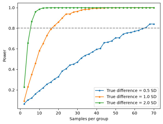
A difference of one SD needs about 18 samples per group, half that difference needs nearly four times as many, and twice the difference only 6. Nothing in this recipe requires normal distributions: the simulated samples can just as well be drawn from pilot measurements, and each simulated experiment can be analyzed with a permutation test, at the cost of more computation.

Two consequences matter for genomics. With three samples per group, the power to detect a difference of one SD is only about 16%, and even a difference of two SD is missed in more than half of the experiments. And when thousands of genes are tested, each gene has to pass a much stricter threshold than $\alpha = 0.05$ (see multiple hypothesis testing); at $\alpha = 0.001$, a difference of one SD needs about 37 samples per group. As each gene has its own difference and variation, an experiment has high power for some genes and low power for others, which is what the next chapter shows on real data.

Overview of the workflow in frequentist testing procedures¶

We are interested in a parameter of a population, such as its mean μ, but can only observe a sample, from which we calculate a statistic, such as the sample mean X̄. The statistic differs from the parameter because of sampling errors, as the sample is only a subset of the population, and because of measurement errors. A statistical model of these errors, such as the null distributions above, is what allows us to use the statistic to draw conclusions about the population parameter.

Volcano Plots and Their Interpretation¶

A volcano plot is a type of scatter plot commonly used in genomics, proteomics, and other fields of biology to display the results of differential expression or differential abundance analysis. The plot provides a clear visual summary of large datasets, making it easier to identify statistically significant changes between two experimental conditions.

On a volcano plot, the x-axis shows the fold change between the two groups, usually as a $\log_2$ value, and the y-axis shows the statistical significance of the change, usually as $-\log_{10}$ of the $p$ value. Features (e.g., genes or proteins) far to the left or right have large fold changes, and features high up have small $p$ values. The most interesting features, with both a large effect size and high statistical confidence, are therefore found in the upper left and upper right corners. The name “volcano plot” comes from the characteristic shape of the point cloud, which resembles an erupting volcano.

Example Script for Generating a Volcano Plot¶

The script below simulates log2 expression values for 1,000 genes in two groups of five samples, and draws a volcano plot. Only about 10% of the genes are differentially expressed, with a random offset between the groups.

import pandas as pd
import matplotlib.pyplot as plt
from scipy.stats import ttest_ind

# Parameters
num_genes = 1000
sample_size = 5
mu, sigma = 4.0, 0.5  # mean and standard deviation of the log2 expression values

# Random number generator
rng = np.random.RandomState(42)

# Generate data for each gene
gene_data = []
for i in range(num_genes):
    # Only about 10% of the genes are differentially expressed,
    # i.e. get a random offset between the two groups
    is_de = rng.rand() < 0.1
    offset = rng.normal(0., 1.) if is_de else 0.
    
    # Generate two samples with the offset
    sample1 = rng.normal(mu, sigma, sample_size)
    sample2 = rng.normal(mu + offset, sigma, sample_size)
    
    # Calculate the log2 fold change as the difference in mean log2 expression
    log2_fc = np.mean(sample2) - np.mean(sample1)
    
    # Perform a t-test to calculate the p value
    _, p_value = ttest_ind(sample1, sample2, alternative='two-sided')
    
    # Store the gene data
    gene_data.append([is_de, log2_fc, p_value])

# Create DataFrame
data = pd.DataFrame(gene_data, columns=['DE', 'Log2FC', 'PValue'])

# Convert p values to -log10(p value)
data['negLog10PValue'] = -np.log10(data['PValue'])

# Mark the genes that pass both the p value and the fold change thresholds
passing = (data['PValue'] < 0.05) & (data['Log2FC'].abs() > 1)

# Create the volcano plot
plt.figure(figsize=(10, 6))
plt.scatter(data.loc[~passing, 'Log2FC'], data.loc[~passing, 'negLog10PValue'], color='grey', alpha=0.6, edgecolors='w', linewidth=0.5)
plt.scatter(data.loc[passing, 'Log2FC'], data.loc[passing, 'negLog10PValue'], color='darkorange', alpha=0.8, edgecolors='w', linewidth=0.5, label='p < 0.05 and |log2 FC| > 1')
plt.axhline(-np.log10(0.05), color='red', linestyle='--', label='p = 0.05')
plt.axvline(-1, color='blue', linestyle='--', label='log2 FC = -1')
plt.axvline(1, color='blue', linestyle='--', label='log2 FC = 1')

plt.xlabel('Log2 Fold Change')
plt.ylabel('-Log10 p value')
plt.title('Volcano Plot of Simulated Gene Data')
plt.legend()
plt.show()

null_genes = ~data['DE']
print(f"Genes without an effect: {null_genes.sum()}, of which {(null_genes & (data['PValue'] < 0.05)).sum()} have p < 0.05 "
      f"and {(null_genes & passing).sum()} pass both thresholds")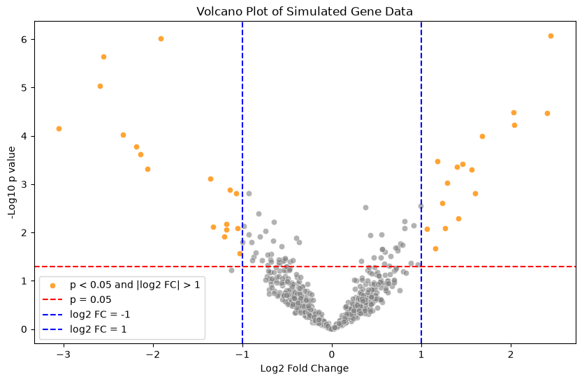

Genes without an effect: 894, of which 45 have p < 0.05 and 2 pass both thresholds

The genes that pass both the $p$ value threshold (red line) and the threshold of $\pm 1$ on the log2 fold change (blue lines) are shown in orange. Of the 894 genes without an effect, 45 nevertheless reach $p < 0.05$; they make up most of the grey points above the red line, and two of them even pass both thresholds. Such false positives are expected when testing many genes, as we have not corrected for multiple testing, something we will discuss in the chapter on multiple hypothesis corrections.