


Linear SVMs
Support Vector Machines (SVMs) are powerful tools for classification tasks, and one of the simplest versions is the Linear SVM. A Linear SVM aims to find the optimal line (or hyperplane in higher dimensions) that separates data points into different classes while maximizing the distance between the classes. This distance is called the margin. In this chapter, we’ll explore how Linear SVMs achieve this.
The Goal of an SVM: Maximum Margin Hyperplane
Imagine we have a set of points that belong to two different classes, represented by the labels +1 and −1. These points, denoted as , where is either +1 or −1, form our training data. Each is a p-dimensional real vector that represents the features of a data point.
The SVM looks for the maximum-margin hyperplane, the hyperplane that divides the data into the two classes while lying as far as possible from the nearest points of both classes. These nearest points are called support vectors.
Defining a Hyperplane
In a p-dimensional space, a hyperplane can be described by the equation:
where:
is the normal vector to the hyperplane, indicating its orientation.
is a parameter that controls the offset of the hyperplane from the origin.
A key objective in Linear SVMs is to find and that maximize the margin—the distance between the hyperplane and the closest data points.
Hard-Margin SVM
If the data is perfectly linearly separable (i.e., there exists a hyperplane that separates the classes without any overlap), we can create two parallel hyperplanes, one for each class. The region between these two hyperplanes is called the margin, and the hyperplane exactly in the middle of this margin is called the maximum-margin hyperplane.
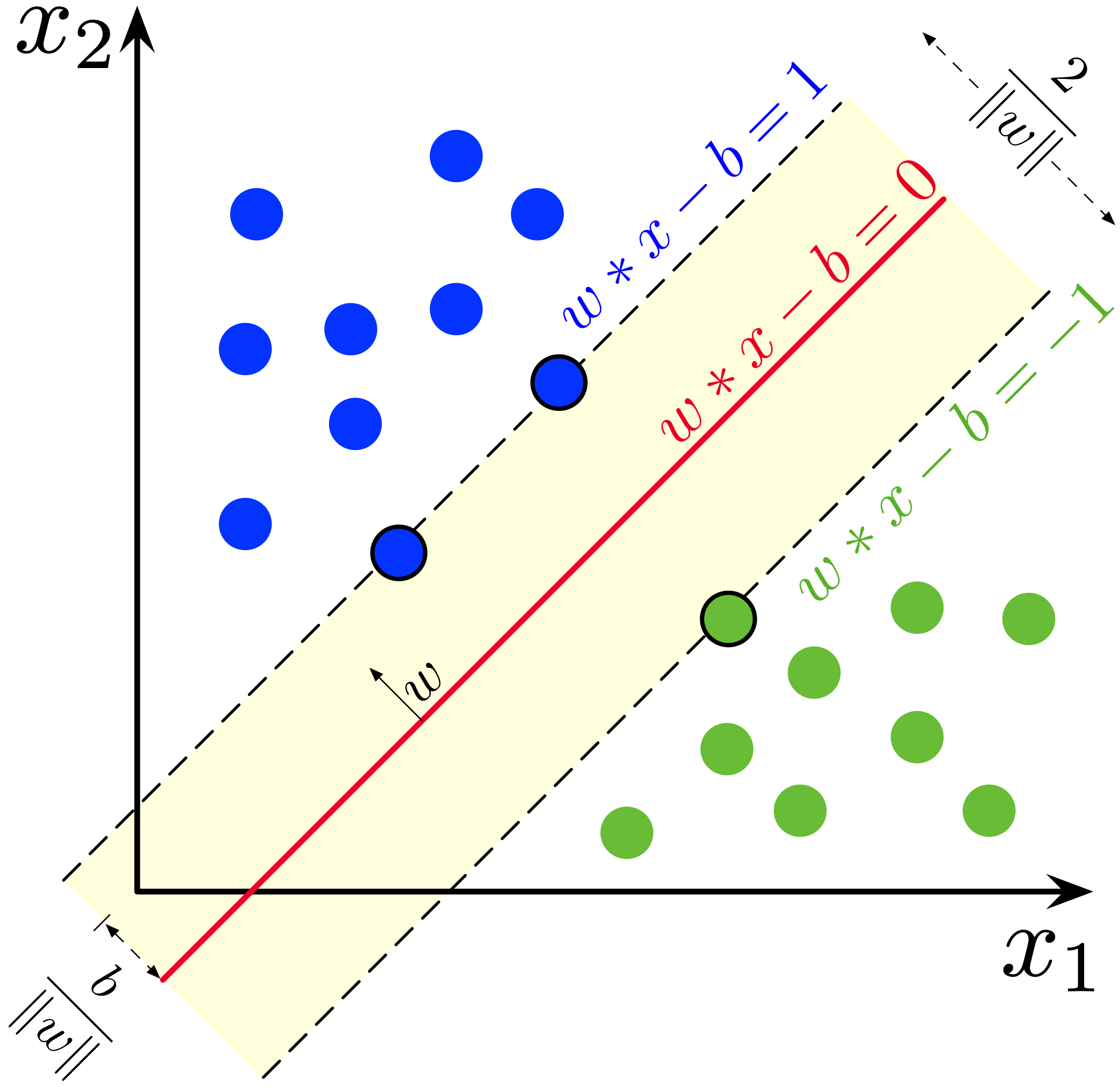
Maximum-margin hyperplane and margins.
Image by Larhmam, CC BY-SA 4.0, via Wikimedia Commons
The equations for the two parallel hyperplanes are:
These equations indicate that the points on or above one hyperplane belong to class +1, and those on or below the other belong to class −1. The distance between the hyperplanes is given by:
To maximize this distance, we need to minimize . At the same time, we need to ensure that every point lies on the correct side of the margin, which leads to the following constraint for each data point:
Optimization Problem
The optimization problem for a hard-margin SVM can be formulated as:
Minimizing gives the same solution as minimizing , but is mathematically more convenient.
Soft-Margin SVM
In real-world scenarios, data is often not perfectly linearly separable. To handle this, we introduce the concept of a soft margin. Instead of forcing every data point to lie outside the margin on its correct side, we allow some points to fall inside the margin or even be misclassified. To measure how much a point violates the margin, we use the hinge loss, which we met in the chapter on classification:
The hinge loss is zero for every point that lies on the correct side of its margin hyperplane, however close to it. It becomes positive once a point enters the margin, and grows linearly the further the point lies on the wrong side; it exceeds 1 for points on the wrong side of the separating hyperplane, i.e. for misclassified points.
The goal for a soft-margin SVM is to minimize the following expression:
Here, is a parameter that controls the trade-off between maximizing the margin and minimizing the classification errors. A smaller value of puts more emphasis on correctly classifying every point, while a larger value allows for a wider margin with some misclassifications. Note that in the example in the next chapter, we will use a slightly different formulation, in terms of a parameter that plays the inverse role of . Rescaling the objective above by turns it into , the form used by scikit-learn’s SVC class, with . A large therefore corresponds to a small , i.e. a strong emphasis on classifying every training point correctly. The LinearSVC class that we use in the next chapter differs slightly: by default it squares the hinge loss of each point, and it also penalizes the offset , but plays the same role.
Support Vectors
An important feature of SVMs is that the maximum-margin hyperplane is determined only by the points that lie closest to it, the support vectors. For a soft-margin SVM, the support vectors also include the points that fall inside the margin or on the wrong side of it. All other points do not affect the hyperplane: removing them, or moving them without entering the margin, leaves the classifier unchanged.
What you should know after reading this chapter
You should be able to:
Define a hyperplane , and explain the roles of the normal vector and the offset .
Explain what the margin of a linear SVM is, and why maximizing the margin width amounts to minimizing .
Write down the hard-margin SVM optimization problem, and use its constraint to judge by hand whether a given point lies on the correct side of the margin.
Explain why a soft margin is needed when the classes are not linearly separable, and calculate the hinge loss for points outside the margin, inside the margin and on the wrong side of the hyperplane.
Write down the soft-margin objective, and explain how trades a wide margin against errors on the training points. Explain why a large in the alternative formulation corresponds to a small .
Define support vectors, and explain why only they determine the maximum-margin hyperplane.