Regression

General¶

The purpose of regression is to model the relationship between a dependent variable (output) and one or more independent variables (inputs). It is one of the most common techniques in statistical modeling, used both to understand and to predict the dependent variable.

Independent and Dependent Variables¶

• Independent variable: Denoted as $\mathbf{x}_i$, these are the input variables or predictors.

• Dependent variable: Denoted as $y_i$, this is the output variable or response we are trying to predict.

A Linear Regression Model¶

With a single independent variable $x_i$, the simplest model is a straight line, $f(x_i) = a x_i + b$, where $a$ is the slope of the line and $b$ is the intercept.

We can write this model in a more general form:

Where:

• $\boldsymbol{\beta} = (b, a)^T$ are the model parameters (intercept and slope),

• $\mathbf{x}_i' = (1, x_i)^T$ is the extended input vector, which includes a constant 1 for the intercept,

• The goal is to find the $\boldsymbol{\beta}$ that best fits the data.

The same form covers several independent variables: then $\mathbf{x}_i' = (1, \mathbf{x}_i^T)^T$, and $\boldsymbol{\beta}$ holds the intercept and one slope per variable.

Residuals¶

In regression, the residual for each data point is the difference between the observed value $y_i$ and the value predicted by the model $f(\mathbf{x}_i)$. The residual for the $i$-th point can be written as:

Residuals give us a way to evaluate how well the model fits the data. A residual close to zero means that the model’s prediction is close to the observed value, while a residual far from zero indicates a larger error.

# When the page runs in the browser (JupyterLite), seaborn is not preinstalled, so we install it first
import sys
if sys.platform == "emscripten":
    import micropip
    await micropip.install("seaborn")

Source

import numpy as np
import matplotlib.pyplot as plt
import seaborn as sns
from scipy.optimize import minimize

# Seaborn settings
sns.set_theme(style="whitegrid")

N = 30  # Number of data points

# Generating random data
rng = np.random.RandomState(0)
x = rng.rand(N)
y_linear = 2 * x - 0.5 + 0.2*rng.randn(N)

# Define a generic loss function for linear models
def loss(params, model_function, x, y):
    return np.sum((y - model_function(x, params))**2)

# Define the linear model function
def linear_model(x, params):
    slope, intercept = params
    return slope * x + intercept

# A function searching for a set of parameters that minimize a given loss function over data,
# starting from a random, but reproducible, initial guess
def minimize_loss(loss, model, x, y, num_params):
    initial_params = np.random.RandomState(0).randn(num_params)
    return minimize(loss, initial_params, args=(model, x, y))

# Minimize the loss function
result_linear = minimize_loss(loss, linear_model, x, y_linear, 2)

# Optimized parameters
slope, intercept = result_linear.x

# Generate prediction line
xfit = np.linspace(0, 1.0, 1000)
yfit_linear = linear_model(xfit, (slope, intercept))

# Plot data, model, and residuals
plt.figure(figsize=(8, 6))
sns.scatterplot(x=x, y=y_linear, label='Data')
plt.plot(xfit, yfit_linear, color='r', label=r'$f(\mathbf{x})$')

# Create a custom legend entry for the residual lines
plt.plot([x[0], x[0]], [y_linear[0], linear_model(x[0], (slope, intercept))], color='blue', label='Residual')

# Draw the residual of each data point as a vertical line
for i in range(len(x)):
    plt.plot([x[i], x[i]], [y_linear[i], linear_model(x[i], (slope, intercept))], color='blue')

plt.xlabel('x')
plt.ylabel('y')
plt.legend()
plt.show()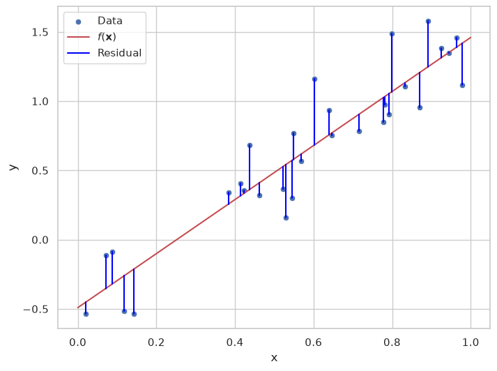

In the figure above, the vertical blue lines are the residuals: they show how much of each data point the model $f(\mathbf{x})$ leaves unexplained.

Least Squares Estimation¶

To fit a function $f(\mathbf{x})$ to the data points $\{(\mathbf{x}_i, y_i)\}_i$, we minimize the sum of squared errors (SSE):

This process is known as least squares. $\mathcal{L}$ is known as a loss function. The loss measures how poorly a model fits the data, and different regression lines have different losses. By minimizing the loss function, we find the function that best fits the data according to the selected loss function.

If the errors $e_i$ are independent and normally distributed with the same variance, the maximum likelihood estimation (MLE) is equivalent to least squares minimization, making this approach optimal under these assumptions.

Minimizing the SSE gives the same parameters as minimizing the more commonly reported mean squared error (MSE), which divides the SSE by the number of data points $N$:

Fit a Linear Model to Data¶

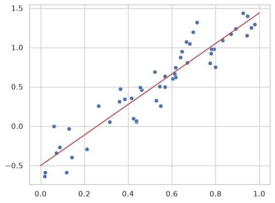
A general pattern in machine learning is to use an optimizer to minimize a loss function. Here, we define the SSE loss explicitly and minimize it with the scipy.optimize.minimize function. Nothing in this procedure is specific to straight lines, so later in this chapter we use the same code to fit non-linear models. Try changing the number of data points N in the code, and see how the fitted slope and intercept change.

from scipy.optimize import minimize
import numpy as np
import seaborn as sns
import matplotlib.pyplot as plt

# Seaborn settings
sns.set_theme(style="whitegrid")

N = 50  # Number of data points

# Generating random data
rng = np.random.RandomState(0) # Any number can be used as seed for the random number generator
x = rng.rand(N)
y_linear = 2 * x - 0.5 + 0.2*rng.randn(N)

# Define a generic loss function for both linear and polynomial models
def loss(params, model_function, x, y):
    return np.sum((y - model_function(x, params))**2)

# Define the linear model function
def linear_model(x, params):
    slope, intercept = params
    return slope * x + intercept

# A function searching for a set of parameters that minimize a given loss function over data,
# starting from a random, but reproducible, initial guess
def minimize_loss(loss, model, x, y, num_params):
    initial_params = np.random.RandomState(0).randn(num_params)
    return minimize(loss, initial_params, args=(model, x, y))

# Minimize the loss function
result_linear = minimize_loss(loss, linear_model, x, y_linear, 2)

# Optimized parameters
slope, intercept = result_linear.x

# Print the optimized slope and intercept
print(f"Optimized slope: {slope}, Optimized intercept: {intercept}")

# Generate prediction line
xfit = np.linspace(0, 1.0, 1000)
yfit_linear = linear_model(xfit, (slope, intercept))

# Plot data and model
sns.scatterplot(x=x, y=y_linear)
plt.plot(xfit, yfit_linear, color='r')
plt.show()

Optimized slope: 1.9385466095021187, Optimized intercept: -0.5014420349612432

Notes on Optimization¶

By default, scipy.optimize.minimize uses the BFGS algorithm, a refinement of gradient descent, to find an optimal set of parameters $(a, b)$. Gradient descent is an iterative algorithm for finding the minimum of a function; here, the function is the loss, and we search for the parameters that minimize it.

Concept of Gradient Descent¶

The basic idea of gradient descent is to start from a guess of the parameters, and then repeatedly change them by a small step in the direction that decreases the loss. That direction is given by the derivative of the loss or, when the model has several parameters, by its gradient. We first look at a model with a single parameter, where the ordinary derivative is enough, and then extend the same code to two parameters.

Gradient Descent with One Parameter¶

If we fix the intercept at $b = 0$, the model becomes a line through the origin, $f(x) = a x$, with the slope $a$ as its only parameter. The loss is then a function of $a$ alone,

and its derivative with respect to $a$ is

The derivative is the slope of the loss curve at the current value of $a$. If it is positive, the loss increases with $a$, so we should decrease $a$. If it is negative, we should increase $a$. Gradient descent therefore takes a step against the derivative,

where the learning rate $\eta$ is a small positive number that sets the step size. Near the minimum, the loss curve flattens and the derivative approaches zero, so the steps become smaller.

Below, we write a general gradient_descent function, which takes a function that calculates the derivative, a starting guess, the learning rate and the number of steps. We use it to fit the slope, starting from $a = 0$.

import numpy as np
import matplotlib.pyplot as plt
from scipy.optimize import minimize

# Data: 30 points from a noisy line with slope 2 and intercept -0.5, as earlier in the chapter
rng = np.random.RandomState(0)
x_ = rng.rand(30)
y_ = 2 * x_ - 0.5 + 0.2*rng.randn(30)

# Gradient descent: start from an initial guess, and repeatedly take a step against the gradient.
# The function works for any number of parameters
def gradient_descent(gradient, params, learning_rate, n_iterations):
    steps = [params]
    for i in range(n_iterations):
        params = params - learning_rate * gradient(params)
        steps.append(params)
    return np.array(steps)

# One parameter: the slope a of a line through the origin, f(x) = a x
def loss_1d(a):
    return np.sum((y_ - a * x_)**2)

def derivative_1d(a):
    return -2 * np.sum(x_ * (y_ - a * x_))

learning_rate = 0.01
n_iterations = 20
steps_1d = gradient_descent(derivative_1d, 0.0, learning_rate, n_iterations)

fig, (ax1, ax2) = plt.subplots(1, 2, figsize=(12, 5))

# Left: the loss as a function of a, with the steps of gradient descent
a_values = np.linspace(-0.5, 3.0, 200)
ax1.plot(a_values, [loss_1d(a) for a in a_values], color='gray', label='Loss')
# The derivative is the slope of the tangent to the loss curve
a0 = steps_1d[0]
tangent_a = np.array([a0 - 0.4, a0 + 0.6])
ax1.plot(tangent_a, loss_1d(a0) + derivative_1d(a0) * (tangent_a - a0), color='black', linestyle=':',
         label='Tangent at the start (slope = derivative)')
ax1.plot(steps_1d, [loss_1d(a) for a in steps_1d], 'o--', color='red', label=f'Gradient descent ({n_iterations} steps)')
ax1.set_xlabel('Slope (a)')
ax1.set_ylabel('Loss')
ax1.legend()

# Right: the data, with the line of each step
ax2.scatter(x_, y_, label='Data')
for a in steps_1d[:-1]:
    ax2.plot([0, 1], [0, a], color='red', alpha=0.2)
ax2.plot([0, 1], [0, steps_1d[-1]], color='red', label=f'Line after {n_iterations} steps')
ax2.set_xlabel('x')
ax2.set_ylabel('y')
ax2.legend()
plt.show()

# The minimum of the same loss, found with scipy's optimizer
a_min = minimize(loss_1d, 0.0).x[0]
print(f"After {n_iterations} steps: slope {steps_1d[-1]:.3f}")
print(f"Minimum of the loss: slope {a_min:.3f}")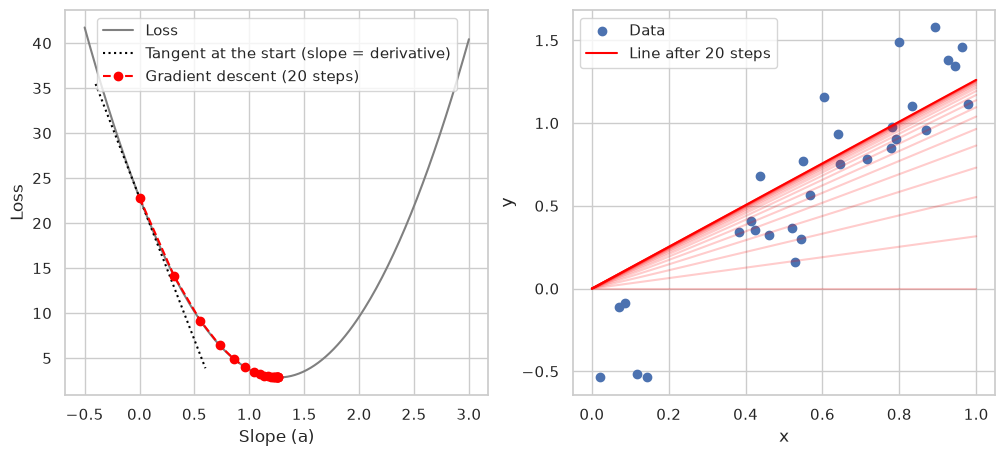

After 20 steps: slope 1.261
Minimum of the loss: slope 1.265

In the left panel, gradient descent starts at $a = 0$, where the loss curve is steep, so the first step is large. The steps then shrink as the curve flattens towards the minimum. In the right panel, the line turns towards the data with each step. Because it is forced through the origin, it cannot follow the data very well, as the data were generated with an intercept of -0.5.

Try changing the learning rate. With learning_rate = 0.07, the steps overshoot the minimum and jump back and forth across it, and with learning_rate = 0.09, every step lands further away from the minimum than the previous one.

Gradient Descent with Two Parameters¶

If we also let the intercept vary, we get back the full model $f(x) = a x + b$, whose loss $\mathcal{L}(a, b)$ depends on two parameters. Instead of a single derivative, we now have one partial derivative per parameter. The partial derivative with respect to $a$ is the ordinary derivative with respect to $a$, calculated as if $b$ were a constant, and vice versa:

With $b = 0$, the first of them is the derivative from the one-parameter case. Together, the partial derivatives form the gradient, a vector that points in the direction in which the loss increases most steeply:

Gradient descent takes a step against the gradient, which means that each parameter is updated with its own partial derivative:

The same holds for any number of parameters. If we collect the parameters in a vector $\boldsymbol{\beta}$, the update rule is

In the code, only the loss and its derivative change: the derivative becomes a gradient function that returns both partial derivatives, and the starting guess becomes a vector $(a, b) = (0, 0)$. The gradient_descent function is the same as before. We draw its steps on a contour plot of the loss as a function of $a$ and $b$.

# Two parameters: the slope a and the intercept b, f(x) = a x + b
def loss_2d(params):
    a, b = params
    return np.sum((y_ - (a * x_ + b))**2)

# The gradient holds one partial derivative per parameter
def gradient_2d(params):
    a, b = params
    residuals = y_ - (a * x_ + b)
    return np.array([-2 * np.sum(x_ * residuals),  # Partial derivative with respect to a
                     -2 * np.sum(residuals)])      # Partial derivative with respect to b

# The same gradient descent function as for one parameter
n_iterations = 100
steps_2d = gradient_descent(gradient_2d, np.array([0.0, 0.0]), learning_rate, n_iterations)

# The minimum of the same loss, found with scipy's optimizer
slope_min, intercept_min = minimize(loss_2d, np.array([0.0, 0.0])).x

# Loss evaluated on a grid of (a, b) values
a_values = np.linspace(-0.5, 3.0, 100)
b_values = np.linspace(-1, 0.5, 100)
loss_grid = np.array([[loss_2d((a, b)) for a in a_values] for b in b_values])

# Plotting the contour plot of the loss function
plt.figure(figsize=(10, 6))
plt.contourf(a_values, b_values, loss_grid, levels=50, cmap='viridis')
plt.colorbar(label='Loss magnitude')
plt.scatter(steps_2d[:, 0], steps_2d[:, 1], color='red', s=50, label=f'Gradient descent ({n_iterations} steps)')
plt.plot(steps_2d[:, 0], steps_2d[:, 1], color='white', linestyle='--', linewidth=1)
plt.scatter([slope_min], [intercept_min], color='white', edgecolor='black', s=60, label='Minimum of the loss')
plt.title('Contour plot of the loss function with Gradient Descent Steps')
plt.xlabel('Slope (a)')
plt.ylabel('Intercept (b)')
plt.legend()
plt.show()

# Output the parameters
print(f"After {n_iterations} steps: slope {steps_2d[-1, 0]:.3f}, intercept {steps_2d[-1, 1]:.3f}")
print(f"Minimum of the loss: slope {slope_min:.3f}, intercept {intercept_min:.3f}")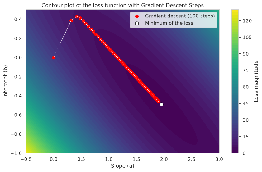

After 100 steps: slope 1.903, intercept -0.462
Minimum of the loss: slope 1.951, intercept -0.491

After 100 steps, gradient descent is still some distance from the minimum: the loss forms a long, narrow valley, and the steps shrink as they follow its nearly flat floor.

Scikit-learn¶

Defining a loss function explicitly and handing it to a general-purpose optimizer is a good way to explain how machine learning works, but it is not how linear regression is usually done in practice. The least-squares problem has an analytical solution, which software packages use instead. In practice, we use a package such as scikit-learn, one of the most popular machine learning libraries in Python, which implements a wide range of supervised and unsupervised methods.

Linear Regression using Scikit-learn¶

Below, we fit the same data as above with scikit-learn’s LinearRegression class.

from sklearn.linear_model import LinearRegression

model = LinearRegression(fit_intercept=True)

model.fit(x[:, np.newaxis], y_linear)

xfit = np.linspace(0, 1, 1000)
yfit = model.predict(xfit[:, np.newaxis])

# Scatter plot with seaborn
sns.scatterplot(x=x, y=y_linear)
plt.plot(xfit, yfit, color='r')
plt.show()

Regression with Basis Functions¶

So far our model has been a straight line, but many relationships are curved. This section shows that the same recipe, choosing a model and minimizing its loss, also fits curved relationships. The trick is to turn each input $x$ into several new features, such as $x$, $x^2$ and $x^3$, and to fit a weighted sum of these features. The model is still linear in its parameters, so the fitting does not change; only the features do. The functions that create the features are called basis functions.

Polynomial Basis Functions¶

A common choice is polynomial basis functions: from each input $x$ we create the terms $x^2$, $x^3$, and so on, which let the model capture curved patterns. Instead of fitting a linear model $y = a x + b$, we then fit a polynomial of degree $n$. This transforms the input space into a higher-dimensional space where the relationship between $x$ and $y$ may be linear, even if it appears non-linear in the original space. Below, we fit a polynomial of degree 7, which has 8 parameters, to 50 data points. Try changing the number of data points N and the degree of the polynomial degree in the code, and see how the fit changes.

import seaborn as sns
import matplotlib.pyplot as plt
import numpy as np

# Seaborn settings
sns.set_theme(style="whitegrid")

N = 50      # Number of data points
degree = 7  # Degree of the polynomial

# Generating random data
rng = np.random.RandomState(1)
x = rng.rand(N)
y_non_linear = np.sin(10.*x) + 0.1 * rng.randn(N)

# Define the polynomial model function, where the degree is given by the number of parameters
def polynomial_model(x, params):
    degree = len(params) - 1
    x_poly = np.vstack([x**i for i in range(degree + 1)]).T
    return np.dot(x_poly, params)


# Optimize the parameters of our model using the same SSE loss function as before.
# A polynomial of degree n has n+1 parameters
result_poly = minimize_loss(loss, polynomial_model, x, y_non_linear, degree + 1)

poly_params = result_poly.x

# Generate fit lines
yfit_poly = polynomial_model(xfit, poly_params)

sns.scatterplot(x=x, y=y_non_linear)
plt.plot(xfit, yfit_poly, color='r')
plt.ylim(-2, 2)  # Fixed range, so that overfitted curves don't hide the data
plt.title("Polynomial Regression Fit")
plt.show()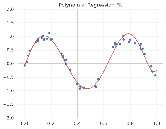

Optional: Gaussian Basis Functions¶

This last part of the chapter is optional reading. Another choice is Gaussian basis functions, also known as radial basis functions (RBF). Each one is a bell-shaped bump around a center, so a weighted sum of them can follow localized, non-linear behavior in the data. Below, we use 11 Gaussian bases and let the optimizer fit not only their weights but also their centers and their common width. That makes the model non-linear in its parameters, but it is still fitted in exactly the same way, by minimizing the SSE.

# Define a Gaussian basis function
def gaussian_basis(x, centers, width):
    return np.exp(-0.5 * ((x[:, np.newaxis] - centers[np.newaxis, :]) / width)**2)

# Define the Gaussian model
def gaussian_model(x, params):
    # Split the params into weights, centers and common width of the bases
    n_bases = len(params)//2
    weights = params[:n_bases]
    centers = params[n_bases:2*n_bases]
    width = params[-1]
    # Calculate the values of each basis for each x
    basis = gaussian_basis(x, centers, width)
    return np.dot(basis, weights)

n_bases = 11  # Number of Gaussian bases to fit to our data

# Optimize the parameters of our model using the same SSE loss function as before
result_gaussian = minimize_loss(loss, gaussian_model, x, y_non_linear, n_bases*2+1)
gaussian_params = result_gaussian.x

yfit_gauss = gaussian_model(xfit, gaussian_params)

# Plot the Gaussian fit
sns.scatterplot(x=x, y=y_non_linear)
plt.plot(xfit, yfit_gauss, color='r')
plt.ylim(-2, 2)
plt.show()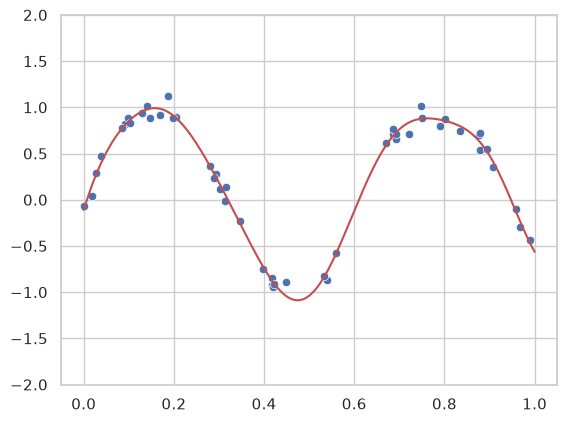

With many basis functions, such flexible models can fit the noise in the data as well as the underlying pattern. The next chapter introduces regularization, which controls model complexity and so counteracts such overfitting.