Regularization

Introduction to Regularization¶

While linear regression works well in many cases, it can suffer from overfitting when the model is flexible relative to the amount of data, for example when a high-degree polynomial is fitted to a few noisy data points. Overfitting occurs when a model captures not only the true underlying pattern but also random fluctuations or noise in the data. This leads to poor generalization on unseen data.

One way to combat overfitting is to apply regularization, which modifies the loss function by adding a penalty for large model parameters. Large parameters are a typical symptom of overfitting: they make the model react strongly to small changes in the input, and so to the noise in the training data. The penalty constrains the model’s flexibility and encourages simpler models that generalize better.

In this chapter, we will introduce two commonly used regularization techniques and their combination:

• Ridge Regression (also known as L2 regularization)

• LASSO Regression (also known as L1 regularization)

• Elastic Net, which combines the two

Ridge Regression (L2 Regularization)¶

In ridge regression, we modify the ordinary least squares loss function by adding a penalty proportional to the square of the parameters’ magnitudes. This penalty discourages large parameters, leading to a smoother model that is less likely to overfit.

The objective function for ridge regression is:

Where:

• $\lambda$ is a regularization parameter that controls the strength of the penalty. When $\lambda = 0$, ridge regression reduces to ordinary least squares. As $\lambda$ increases, the penalty becomes stronger.

• $\beta_j$ are the model parameters. By convention the intercept is left out of the penalty, so that the fit does not depend on where the origin of $y$ happens to lie. Note that our own implementations below penalize every coefficient of the polynomial model, including its constant term, while scikit-learn’s ElasticNet, used at the end of the chapter, leaves its intercept unpenalized.

Ridge Regression by Explicit Loss Minimization¶

Here we implement the ridge loss explicitly and minimize it numerically, so that the penalty term stays visible. In practice you would normally reach for scikit-learn’s Ridge class. As data, we use 20 noisy points from a polynomial curve, and we fit a polynomial of degree 7 to them, with and without the penalty.

# When the page runs in the browser (JupyterLite), seaborn is not preinstalled, so we install it first
import sys
if sys.platform == "emscripten":
    import micropip
    await micropip.install("seaborn")

from scipy.optimize import minimize
import numpy as np
import seaborn as sns
import matplotlib.pyplot as plt

# Generate synthetic data
rng = np.random.RandomState(16)
N = 20
x = rng.rand(N)
y_non_linear = 4 * x**2 - 10 * x**4 + 6 * x**6 + 0.1 * rng.randn(N)

# Define the polynomial model function
def polynomial_model(x, params, degree=7):
    x_poly = np.vstack([x**i for i in range(degree + 1)]).T
    return np.dot(x_poly, params)

# Minimize a loss function, starting from a random, but reproducible, initial guess
def minimize_loss(loss, model, x, y, num_params):
    initial_params = np.random.RandomState(0).randn(num_params)
    return minimize(loss, initial_params, args=(model, x, y))

# Residual sum of squares (RSS), i.e. the SSE of the previous chapter
def rss_loss(params, model_function, X, y):
    predictions = model_function(X, params)  # Predicted values
    residual_sum_squares = np.sum((y - predictions) ** 2)  # RSS
    return residual_sum_squares

# Define ridge loss function
def ridge_loss(params, model_function, X, y, alpha=0.1):
    residual_sum_squares = rss_loss(params, model_function, X, y)  # RSS
    l2_penalty = alpha * np.sum(params**2)
    return residual_sum_squares + l2_penalty

# Optimize the parameters of our model using the RSS and the ridge loss functions
result_poly_rss = minimize_loss(rss_loss, polynomial_model, x, y_non_linear, 8)
result_poly_ridge = minimize_loss(ridge_loss, polynomial_model, x, y_non_linear, 8)

poly_params_rss = result_poly_rss.x
poly_params_ridge = result_poly_ridge.x

# Generate fit lines
xfit = np.linspace(np.min(x), np.max(x), 1000)
yfit_poly_rss = polynomial_model(xfit, poly_params_rss)
yfit_poly_ridge = polynomial_model(xfit, poly_params_ridge)

sns.scatterplot(x=x, y=y_non_linear, label="Data")
plt.plot(xfit, yfit_poly_rss, color='r', label="RSS")
plt.plot(xfit, yfit_poly_ridge, color='b', label="Ridge")
plt.legend()
plt.show()

print("Polynomial parameters (RSS):", poly_params_rss)
print("Polynomial parameters (Ridge):", poly_params_ridge)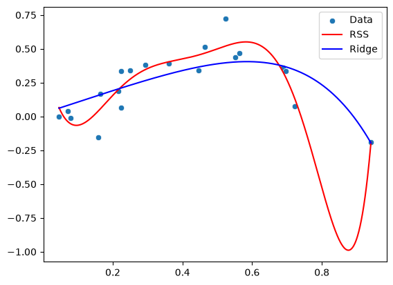

Polynomial parameters (RSS): [ 5.47824138e-01 -1.59883737e+01  1.38372146e+02 -4.58078397e+02
  6.14035870e+02 -4.26836709e+01 -5.89981334e+02  3.56831336e+02]
Polynomial parameters (Ridge): [ 0.02248597  0.84009749  0.07809837 -0.27339012 -0.35827061 -0.33258107
 -0.27178283 -0.20743716]

In the code, alpha plays the role of $\lambda$.

LASSO Regression (L1 Regularization)¶

LASSO regression (Least Absolute Shrinkage and Selection Operator) is another regularization technique. Instead of penalizing the sum of squared parameters, LASSO penalizes the sum of the absolute values of the parameters.

The objective function for LASSO regression is:

Where:

• $\lambda$ again controls the regularization strength.

• The absolute value penalty leads to sparse models, meaning that LASSO can perform feature selection by setting some parameters exactly to zero.

LASSO Regression by Explicit Loss Minimization¶

Here we implement the LASSO loss explicitly and minimize it numerically. Note that this general-purpose optimizer drives coefficients close to zero without setting them exactly to zero. Solvers designed for LASSO, such as the coordinate descent used by scikit-learn’s Lasso class or least-angle regression, do produce exact zeros.

import numpy as np
import matplotlib.pyplot as plt
import seaborn as sns
from scipy.optimize import minimize

# Define LASSO loss function
def lasso_loss(params, model_function, X, y, alpha=0.1):
    residual_sum_squares = rss_loss(params, model_function, X, y)  # RSS
    l1_penalty = alpha * np.sum(np.abs(params))  # L1 regularization
    return residual_sum_squares + l1_penalty

# Optimize the parameters of our model using the lasso loss function
result_poly_lasso = minimize_loss(lasso_loss, polynomial_model, x, y_non_linear, 8)

poly_params_lasso = result_poly_lasso.x

# Generate fit lines
yfit_poly_lasso = polynomial_model(xfit, poly_params_lasso)

sns.scatterplot(x=x, y=y_non_linear, label="Data")
plt.plot(xfit, yfit_poly_rss, color='r', label="RSS")
plt.plot(xfit, yfit_poly_lasso, color='b', label="LASSO")
plt.legend()
plt.show()

# Print parameters
print("Polynomial parameters (RSS):", poly_params_rss)
print("Polynomial parameters (LASSO):", poly_params_lasso)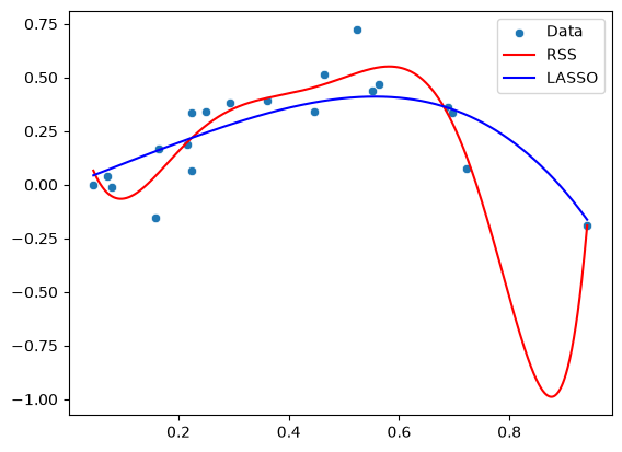

Polynomial parameters (RSS): [ 5.47824138e-01 -1.59883737e+01  1.38372146e+02 -4.58078397e+02
  6.14035870e+02 -4.26836709e+01 -5.89981334e+02  3.56831336e+02]
Polynomial parameters (LASSO): [-2.61105183e-03  1.01056480e+00 -3.25495973e-04 -1.95542003e-01
 -1.19779462e+00 -1.16530979e-02  2.19927836e-03 -2.58220514e-03]

Comparing Ridge and LASSO¶

Ridge regression shrinks all parameters but rarely sets any of them exactly to zero, so every feature stays in the model with a reduced influence. LASSO can shrink parameters all the way to zero and so performs feature selection. Ridge is therefore a natural choice when you believe that most features are relevant, and LASSO when you suspect that only a few of them are.

Elastic Net: Combining Ridge and LASSO¶

Elastic Net includes both the L1 and the L2 penalty:

Here, $\lambda_1$ and $\lambda_2$ set the strengths of the L1 and the L2 penalty. Elastic Net is particularly useful when features are correlated, as it encourages a grouping effect, where correlated features tend to get similar parameters.

Elastic Net Using Scikit-learn¶

scikit-learn’s ElasticNet class writes the penalty with an overall strength $\alpha$ (alpha) and a mixing parameter $\rho$ (l1_ratio), and it divides the squared errors by $2N$. With $N$ data points, this corresponds to $\lambda_1 = 2N\alpha\rho$ and $\lambda_2 = N\alpha(1-\rho)$ in the formula above, so the settings below, with $N = 20$, give $\lambda_1 = 0.1$ and $\lambda_2 = 0.05$. ElasticNet fits its own, unpenalized, intercept, so we leave the constant term out of the polynomial features.

from sklearn.linear_model import ElasticNet

# Fit Elastic Net model on the polynomial features x, x^2, ..., x^7
x_poly = np.vstack([x**i for i in range(1, 8)]).T
elastic_net_model = ElasticNet(alpha=0.005, l1_ratio=0.5)  # l1_ratio controls the balance between L1 and L2 regularization
elastic_net_model.fit(x_poly, y_non_linear)

# Predict and plot
x_poly_fit = np.vstack([xfit**i for i in range(1, 8)]).T
yfit_elastic_net = elastic_net_model.predict(x_poly_fit)

sns.scatterplot(x=x, y=y_non_linear, label="Data")
plt.plot(xfit, yfit_elastic_net, color='m', label="Elastic net")
plt.legend()
plt.show()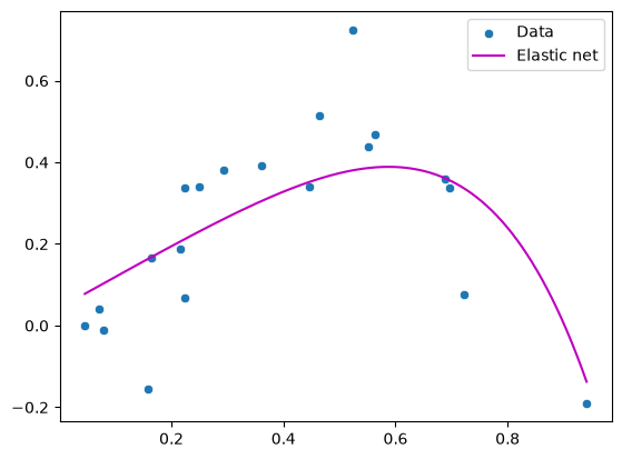

Why “L1” and “L2” Regularization?¶

The labels “L1” and “L2” come from the notation of vector norms in mathematics. A norm on a vector space is a function that assigns a non-negative length or size to each vector and satisfies certain axioms (positivity, homogeneity, triangle inequality). The L1 norm (also written $\ell_1$-norm) of the parameter vector $\boldsymbol{\beta} = (\beta_1, \beta_2, \dots, \beta_p)$ is

The L2 norm (also written $\ell_2$-norm) is

which corresponds geometrically to the Euclidean length of the vector. The LASSO penalty is thus $\lambda \|\boldsymbol{\beta}\|_1$, and the ridge penalty is $\lambda \|\boldsymbol{\beta}\|_2^2$, the squared L2 norm.