Pathway Analysis - Data Science for Biotechnology students

Introduction¶

A typical output from a high-throughput experiment is a list of genes, transcripts, or proteins. Given this list, one might want to identify common functions among these analytes. Here, pathway analysis has become a go-to method for associating functions with experimental findings. A pathway represents a set of biochemical reactions and interactions that take place within a cell or organism, involving metabolites, genes, and proteins. Understanding these pathways allows researchers to link molecular changes to phenotypic outcomes, such as disease states or responses to treatment.

Pathway Databases¶

Examples of commonly used pathway databases include KEGG, Reactome, WikiPathways, and BioCyc, which provide curated pathways for metabolic and signaling processes across various organisms. For specialized needs, researchers use databases like MetaCyc for metabolic pathways, SIGNOR for signaling networks, and CTD for studying toxicogenomic interactions. Although not formally a pathway database, Gene Ontology (GO) is often utilized alongside pathway-based methods to identify enriched biological processes, cellular components, and molecular functions from gene or protein lists.

KEGG¶

The Kyoto Encyclopedia of Genes and Genomes (KEGG) is a manually curated database that integrates genomic, chemical, and systemic functional information into comprehensive pathway maps, including metabolic and regulatory pathways, drawn as graphical diagrams of the molecular interactions.

Reactome¶

Reactome is a detailed, open-source, manually curated knowledge base that provides information about cellular processes like metabolic reactions and immune system functions. Reactome focuses on the relationships between genes, proteins, and other molecules, offering more granular details about molecular interactions than KEGG.

Over-Representation Analysis (ORA)¶

One of the basic approaches to pathway analysis is Over-Representation Analysis (ORA). ORA identifies pathways that are statistically overrepresented in a list of differentially expressed genes or proteins compared to what would be expected by chance.

Fisher’s Exact Test¶

A common statistical method used for ORA is Fisher’s exact test, which is designed to determine if there are nonrandom associations between two categorical variables. In the context of pathway analysis, Fisher’s exact test can be used to assess whether the number of genes from a given pathway in the input list is significantly larger than what would be expected by random chance. The null hypothesis in this context is that a gene in the pathway is no more likely to appear in the gene list than a gene outside the pathway, i.e. that the odds ratio $ad/bc$ equals 1.

Consider the following contingency table:

	In Pathway	Not in Pathway	Sum
In Gene List	$a$	$b$	$a+b$
Not in Gene List	$c$	$d$	$c+d$
All Genes	$a+c$	$b+d$	$a+b+c+d$

We expect the overlap between the pathway and a gene list, as a fraction of all genes, to be just the product of the fraction of genes in the pathway and the fraction of genes in the gene list. Any excess over that fraction is an enrichment. To calculate the significance of such an enrichment, we start by considering the number of combinations of ways to pick genes from the input list and pathway using choose notation. The probability of observing a particular outcome can be expressed as:

P(X = a) = \frac{\binom{a+b}{a} \binom{c+d}{c}}{\binom{a+b+c+d}{a+c}}

(1)

Expanding the binomial expressions, we have:

P(X = a) = \frac{\frac{(a+b)!}{a! b!} \cdot \frac{(c+d)!}{c! d!}}{\frac{(a+b+c+d)!}{(a+c)! (b+d)!}}

(2)

Simplifying this further, we get:

P(X = a) = \frac{(a+b)! (c+d)! (a+c)! (b+d)!}{a! b! c! d! (a+b+c+d)!}

(3)

This represents the probability of picking $a$ genes in, and $b$ genes not in the pathway from the gene list. The $p$ value is the probability of an overlap at least as large as the observed one, given the row and column sums of the table. We therefore sum over the observed outcome and all outcomes that are more extreme in the direction of over-representation:

p = \sum_{x \geq a} P(X = x)

(4)

import matplotlib.pyplot as plt
import numpy as np

# Define fixed fractions for illustration
fraction_in_pathway = 0.2  # e.g., 20% of the total genes are in the pathway
fraction_in_gene_list = 0.3  # e.g., 30% of the total genes are in the gene list

# Create the plot
plt.figure(figsize=(8, 6))

# Plot the lines representing the fractions, extended to the axes
plt.plot([0, 1], [fraction_in_gene_list, fraction_in_gene_list], 'k--', label="Fraction in Gene List")  # horizontal line
plt.plot([fraction_in_pathway, fraction_in_pathway], [0, 1], 'k:', label="Fraction in Pathway")  # vertical line

# Highlight the overlap region
plt.fill_betweenx([0, fraction_in_gene_list], 0, fraction_in_pathway, color="lightblue", label="Expected Overlap")

# Add text annotations
plt.text(fraction_in_pathway / 2, fraction_in_gene_list / 2, "Overlap genes",
         color="blue", ha="center", va="center", fontsize=12, bbox=dict(facecolor="white", alpha=0.8, edgecolor="none"))

# Format the plot
plt.title("Illustration of Expected Overlap", fontsize=14)
plt.xlabel("Fraction of Genes in Pathway", fontsize=12)
plt.ylabel("Fraction of Genes in Gene List", fontsize=12)
plt.xlim(0, 1)
plt.ylim(0, 1)
plt.legend()
plt.grid(True, linestyle="--", alpha=0.7)
plt.tight_layout()

# Show the plot
plt.show()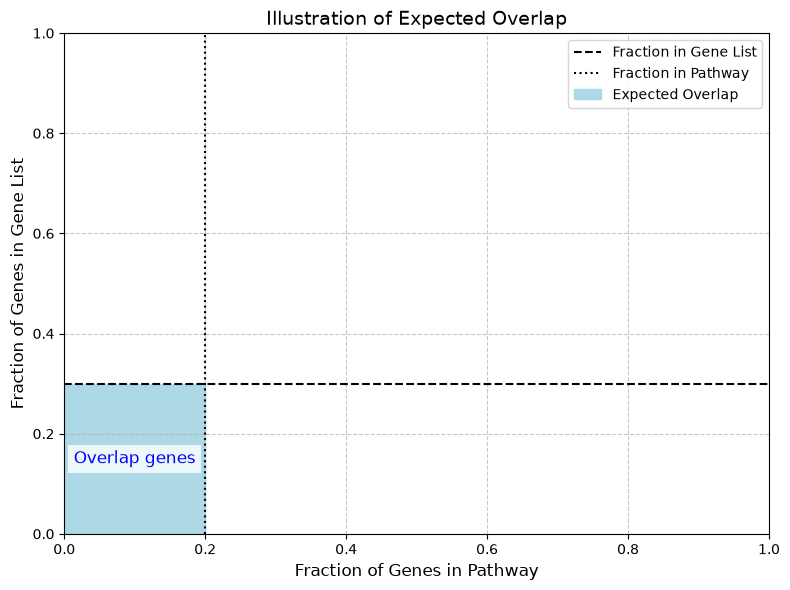

Above is an illustration of the expected overlap (6%) of a pathway consisting of 20% of all genes and a gene list of 30% of all genes.

Gene Set Enrichment Analysis (GSEA)¶

Gene Set Enrichment Analysis (GSEA) is a more sophisticated pathway analysis method compared to ORA, in that it makes use of quantitative information. Unlike ORA, which relies on a predefined threshold to determine differentially expressed genes, GSEA considers the entire list of genes, sorted by differential abundance, and asks whether the genes of a given pathway tend to be overrepresented among the most up- or down-regulated genes, i.e. at the top or bottom of the ranked list.

Enrichment Score¶

GSEA works by calculating an enrichment score (ES), which quantifies the maximal difference between the observed and expected cumulative distributions of gene ranks of the genes in a pathway; i.e. how unevenly distributed the genes from the gene set of interest appear in the list of all genes. Starting at the top of the ranked gene list, an enrichment score is computed by walking down the list, increasing when a gene is in the gene set and decreasing otherwise.

Here is an illustration of the enrichment score. We generate a normally-distributed dataset of 30 samples covering 130 genes, of which 100 form an unregulated background and the remaining 30 belong to two pathways of 15 genes each. The pathway genes are simulated as “regulated”, i.e. given an additional random offset between the “Healthy” and the “Sick” samples, but in opposite directions for the two pathways. GSEA ranks the data and displays the position of the genes of a pathway as colored vertical lines among the remaining genes. If the colored vertical lines were evenly distributed, the enrichment of the pathway genes would be close to zero. Here, the genes of one pathway fall preferentially at the top (left) of the ranked list, driving the running sum upwards and giving a large positive enrichment score, while the genes of the other fall preferentially at the bottom (right), giving a large negative enrichment score.

import numpy as np
import pandas as pd
import gseapy as gp

# Seed for reproducibility
np.random.seed(42)

n_genes_in_pathway = 15
n_genes_in_background = 100
n_samples_per_group = 15

pathway1_genes = { f"Pathway1Gene{i}" for i in range(1, n_genes_in_pathway + 1 ) }
pathway2_genes = { f"Pathway2Gene{i}" for i in range(1, n_genes_in_pathway + 1 ) }
pathway_db = {"Pathway1" : pathway1_genes, "Pathway2" : pathway2_genes }
genes = list(pathway1_genes) + list(pathway2_genes) + [f"Gene{i}" for i in range(1, n_genes_in_background + 1 )]
samples = [f"Sample{j}" for j in range(1, 2*n_samples_per_group + 1)]
fake_data = pd.DataFrame(np.random.normal(0, 1, size=(len(genes), len(samples))), index=genes, columns=samples)

for gene in pathway1_genes:
    if gene in fake_data.index:
        # Make pathway1 genes have higher values in the first half of samples
        fake_data.loc[gene, fake_data.columns[:n_samples_per_group]] += np.random.normal(0.5, 0.5, size=n_samples_per_group)
for gene in pathway2_genes:
    if gene in fake_data.index:
        # Make pathway2 genes have higher values in the second half of samples
        fake_data.loc[gene, fake_data.columns[n_samples_per_group:2*n_samples_per_group]] += np.random.normal(0.5, 0.5, size=n_samples_per_group)

labels = ["Healthy"]*n_samples_per_group + ["Sick"]*n_samples_per_group

gs = gp.GSEA(data=fake_data, 
                 gene_sets=pathway_db, 
                 classes=labels,
                 permutation_type='phenotype', # null from permutations of class labels
                 permutation_num=2000, # number of permutations in the null distribution
                 outdir=None,  # do not write output to disk
                 no_plot=True, # Skip plotting
                 method='signal_to_noise',
                 threads=4, # Number of allowed parallel processes
                 seed=42)
gs.run()
gs.plot(["Pathway1", "Pathway2"], show_ranking=False)
gs.res2d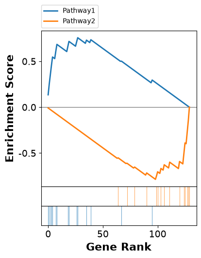

To assess the statistical significance of the observed enrichment score, GSEA uses a sampling distribution of ES obtained through permutation. The phenotype labels are shuffled many times; for each shuffle the genes are re-ranked and the ES recomputed, generating a background distribution of ES values which can then be used to calculate the $p$ value for the observed enrichment score. Permuting the phenotype rather than the ranked gene list preserves the correlation structure between genes, which is why it is the recommended null.

For a more detailed explanation of the enrichment score, please check out the original paper, Subramanian et al..

Kolmogorov-Smirnov (KS) Test¶

The Kolmogorov-Smirnov (KS) test is a non-parametric test that measures the maximum deviation between the observed cumulative distribution of the gene set and the expected distribution under the null hypothesis. The GSEA enrichment score, the maximum deviation of the running sum as we move down the ranked list, is a statistic of this kind.

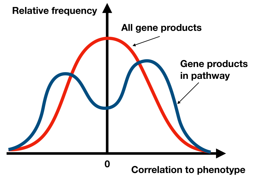
Figure 1:GSEA uses a KS-like test to evaluate whether the genes of a pathway differ significantly from all other genes in how they correlate with the phenotype (e.g. “Healthy” or “Disease”).

It is not the classic KS statistic, though: by default the running sum is weighted, stepping up by $|r_j|/\sum_{\rm hits}|r_j|$ at each pathway gene, where $r_j$ is that gene’s ranking metric, and down by $1/(N-N_H)$ at each of the remaining genes ( $N$ is the number of genes in the ranked list and $N_H$ the number of them in the pathway), so that strongly ranked genes contribute more than marginal ones. Only the unweighted variant reduces to the classic KS statistic. Because this weighted statistic has no closed-form null distribution, and because the genes of a pathway are correlated rather than independent as the KS asymptotics assume, significance is assessed by permutation rather than read off from KS tables. GSEA also corrects for multiple testing by calculating false discovery rates (FDRs).