


Introduction
In the previous chapters a pathway was a set of genes. This chapter treats metabolism as a quantitative network. Metabolic reactions do not merely group genes together — they consume and produce metabolites in fixed stoichiometric proportions, and the rates at which they run must be compatible with each other. By writing down these constraints explicitly, we can simulate metabolism: predict how fast a cell can grow, which nutrients it needs, which genes it cannot survive without, and how it will reroute its metabolism when a gene is knocked out or a nutrient runs out.
The rate at which a reaction converts substrates into products is called its flux, typically measured in mmol per gram dry weight of cells per hour (mmol gDW⁻¹ h⁻¹). In principle, fluxes could be computed from enzyme kinetics. For a single enzyme, Michaelis–Menten kinetics gives the flux as
but this requires knowing , , enzyme and metabolite concentrations for every reaction in the cell — thousands of parameters that are difficult or impossible to measure. Flux balance analysis (FBA) takes a radically more economical approach: instead of trying to compute the one true flux distribution from kinetics, it asks which flux distributions are possible given the stoichiometry of the network, and then selects among them with an optimality principle (see the primer by Orth, Thiele and Palsson). The only inputs needed are the reaction stoichiometries and a handful of measured exchange rates — no kinetic parameters at all.
Genome-Scale Metabolic Models
The networks on which FBA operates are called genome-scale metabolic models (GEMs). A GEM is a mathematical reconstruction of all metabolic reactions known to occur in an organism, assembled from its genome annotation together with pathway databases such as KEGG, Reactome and organism-specific literature. The reconstruction process is analogous to genome assembly: just as a genome is assembled from sequence reads, an organism’s reactome is assembled from individual biochemical reactions, each linked to the enzyme that catalyzes it and the gene that encodes the enzyme.
A GEM contains three layers of information:
Reactions and metabolites, with exact, mass-balanced stoichiometry. Metabolites in different cellular compartments (cytosol, mitochondria, extracellular space, …) are treated as distinct species, so transport steps between compartments are themselves reactions.
Gene–protein–reaction (GPR) rules that connect each reaction to the gene(s) whose products catalyze it. The rules use Boolean logic:
GENE1 and GENE2means the enzyme is a complex requiring both subunits, whileGENE1 or GENE2means two isozymes can each carry the reaction independently.Bounds and exchange reactions that describe which metabolites the cell can import from or export to its environment, and how fast.
The first GEM, for Haemophilus influenzae, was published in 1999; today models exist for thousands of organisms, from E. coli (the best curated model, iML1515) to yeast and human. Human metabolism is described by generic models such as Recon3D and Human-GEM with on the order of 13,000 reactions, 8,000 metabolites and 3,000 genes. An overview of available models and their applications is given by Gu et al..
It is worth stressing what distinguishes a GEM from a pathway map such as those in KEGG. A pathway map records the topology of metabolism — which metabolites are connected by which reactions. A GEM additionally records the stoichiometry, and this makes all the difference: a topological analysis of glycolysis would tell us that glucose is eventually converted to pyruvate, but only the stoichiometric model knows that each glucose yields exactly two pyruvate, two net ATP, and that the pathway stalls without a way to regenerate NAD⁺. Empirically, model-based predictions of gene essentiality agree considerably better with experimental knockout screens than purely topological measures, such as how many connections a gene’s reactions have in the network.
The Stoichiometric Matrix
The mathematical core of a GEM is its stoichiometric matrix , with one row per metabolite and one column per reaction. The entry is the stoichiometric coefficient of metabolite in reaction : negative if the metabolite is consumed, positive if it is produced, and zero if it does not participate. Almost all entries are zero, since a typical reaction involves only a handful of metabolites.
Throughout this chapter we will use a deliberately small model of core energy metabolism — a cartoon of glycolysis, respiration and fermentation:
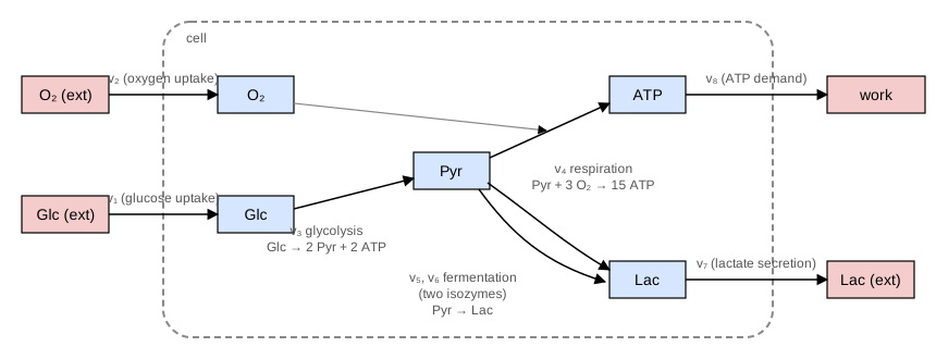
Figure 1:A toy model of core energy metabolism. Blue boxes are internal metabolites. Red boxes lie outside the cell boundary (dashed) and are connected to it through exchange reactions: the external metabolites, and “work”, the sink that consumes ATP. The gray arrow indicates that oxygen enters as a co-substrate of the respiration reaction. The 2 ATP made by glycolysis appear only in its reaction label.
The model has five metabolites and eight reactions:
| Reaction | Chemistry | Interpretation |
|---|---|---|
| Glc | glucose uptake (exchange) | |
| O₂ | oxygen uptake (exchange) | |
| Glc 2 Pyr + 2 ATP | glycolysis (lumped) | |
| Pyr + 3 O₂ 15 ATP | respiration (lumped) | |
| Pyr Lac | fermentation, isozyme 1 | |
| Pyr Lac | fermentation, isozyme 2 | |
| Lac | lactate secretion (exchange) | |
| ATP | ATP demand (exchange) |
Whole pathways are lumped into single reactions, and side metabolites (CO₂, water, NADH) are omitted, but the ATP yields are roughly right: complete oxidation of one glucose yields ATP, while fermentation to lactate yields only the 2 ATP of glycolysis. Reactions , , and are exchange reactions: they appear chemically unbalanced (“Glc appears from nothing”) because they represent transport across the boundary of the system. Every model needs them — without exchange reactions, the steady-state assumption introduced below would force all fluxes to zero. The two parallel fermentation reactions and represent two isozymes, i.e. a GPR rule of the form LDHA or LDHB.
The stoichiometric matrix of this model is
The Steady-State Assumption
Let be the vector of metabolite concentrations and the vector of fluxes. The stoichiometric matrix connects the two: the concentrations change according to
FBA now makes its central assumption, the pseudo-steady state: over the time scale of interest, internal metabolite concentrations do not change, because metabolism operates much faster than the processes that alter cellular composition (growth, regulation). Every internal metabolite is produced exactly as fast as it is consumed:
This is a strong simplification — it makes the model blind to metabolite accumulation and to dynamics — but it is what frees us from kinetics: the equation involves only stoichiometry and fluxes, not concentrations or rate constants.
Together with bounds on each flux,
the steady-state equation defines the space of feasible flux distributions. Bounds encode reaction irreversibility ( for irreversible reactions), maximal uptake rates of nutrients (e.g. glucose uptake at most 10 mmol gDW⁻¹ h⁻¹), and knockouts ().
Note that the system is underdetermined: a genome-scale model has far more reactions (unknowns) than metabolites (equations) — the toy model has 8 unknowns and 5 equations, Human-GEM has some 13,000 unknowns and 8,000 equations. There is therefore no unique solution but a whole continuum of feasible flux distributions, geometrically a convex polytope in flux space. Constraint-based modeling embraces this: rather than pinning down the flux state, the constraints delimit everything the network can do.
FBA as Linear Programming
To select a biologically meaningful flux distribution from the feasible space, FBA assumes that evolution has tuned metabolism to be (near-)optimal for some cellular objective , a linear combination of fluxes. FBA is then the optimization problem
which is a linear program (LP): the objective and all constraints are linear in . Linear programs of enormous size can be solved efficiently and to global optimality — this is what makes FBA feasible at genome scale, in contrast to kinetic models.
The choice of objective is a modeling decision. For microbes, the standard objective is flux through a biomass reaction — an artificial reaction that drains amino acids, nucleotides, lipids and energy in the proportions needed to build one gram of cell, so that maximizing it means maximizing growth rate. Fast-growing cells such as bacteria or tumor cells are plausibly selected for growth; for differentiated human cells one instead uses objectives such as ATP production (muscle), neurotransmitter synthesis (neurons), or lipid storage (adipocytes). Note that the objective must be something the cell produces: maximizing a nutrient uptake flux is not meaningful, since the optimum would simply sit at whatever upper bound we imposed on the uptake, telling us nothing.
A Worked Example
Let us put the toy model to work with nothing but numpy and scipy’s linear-programming routine. We maximize ATP production () under a fixed glucose supply and ask what happens when oxygen becomes scarce.
import numpy as np
import pandas as pd
from scipy.optimize import linprog

metabolites = ["Glc", "O2", "Pyr", "ATP", "Lac"]
reactions = ["glc_uptake", "o2_uptake", "glycolysis", "respiration",
             "ferm_iso1", "ferm_iso2", "lac_secretion", "atp_demand"]

S = np.array([
    # v1  v2  v3  v4  v5  v6  v7  v8
    [  1,  0, -1,  0,  0,  0,  0,  0],   # Glc
    [  0,  1,  0, -3,  0,  0,  0,  0],   # O2
    [  0,  0,  2, -1, -1, -1,  0,  0],   # Pyr
    [  0,  0,  2, 15,  0,  0,  0, -1],   # ATP
    [  0,  0,  0,  0,  1,  1, -1,  0],   # Lac
])

def fba(bounds, c):
    """Maximize c @ v subject to S v = 0 and lb <= v <= ub."""
    res = linprog(-np.asarray(c), A_eq=S, b_eq=np.zeros(len(metabolites)),
                  bounds=bounds, method="highs")
    assert res.success, res.message
    return res.x + 0.0, -res.fun + 0.0  # + 0.0 turns -0.0 into 0.0

objective = np.zeros(len(reactions))
objective[reactions.index("atp_demand")] = 1.0

def make_bounds(glc_max=10.0, o2_max=np.inf):
    bounds = [(0.0, None)] * len(reactions)  # all reactions irreversible
    bounds[reactions.index("glc_uptake")] = (0.0, glc_max)
    bounds[reactions.index("o2_uptake")] = (0.0, o2_max)
    return bounds

flux_aerobic, atp_aerobic = fba(make_bounds(o2_max=np.inf), objective)
flux_limited, atp_limited = fba(make_bounds(o2_max=15.0), objective)

print(pd.DataFrame({"plenty of O2": flux_aerobic,
                    "O2 limited": flux_limited}, index=reactions))
print(f"\nMaximal ATP production: {atp_aerobic:.0f} vs {atp_limited:.0f}")
plenty of O2 O2 limited
glc_uptake 10.0 10.0
o2_uptake 60.0 15.0
glycolysis 10.0 10.0
respiration 20.0 5.0
ferm_iso1 0.0 15.0
ferm_iso2 0.0 0.0
lac_secretion 0.0 15.0
atp_demand 320.0 95.0
Maximal ATP production: 320 vs 95
With plenty of oxygen, the optimal strategy is pure respiration: all 20 pyruvate produced from 10 glucose are oxidized, yielding 320 ATP, and no lactate is secreted. When oxygen uptake is capped at 15, respiration can only handle 5 pyruvate; the remaining 15 overflow into fermentation and leave the cell as lactate, and the ATP yield collapses to 95. If we read the oxygen cap as a limit on the cell’s respiratory capacity rather than on oxygen itself, this is overflow metabolism: once respiration is saturated, the remaining pyruvate is fermented even though oxygen is available. Examples are yeast fermenting to ethanol, E. coli secreting acetate, and the Warburg effect, the large lactate secretion of tumor cells; constraint-based models of cancer metabolism build directly on this logic.
import matplotlib.pyplot as plt

x = np.arange(len(reactions))
w = 0.38
plt.figure(figsize=(8, 4))
plt.bar(x - w/2, flux_aerobic, w, label="plenty of O2")
plt.bar(x + w/2, flux_limited, w, label="O2 limited")
plt.xticks(x, reactions, rotation=30, ha="right")
plt.ylabel("flux (mmol gDW$^{-1}$ h$^{-1}$)")
plt.legend()
plt.tight_layout()
plt.show()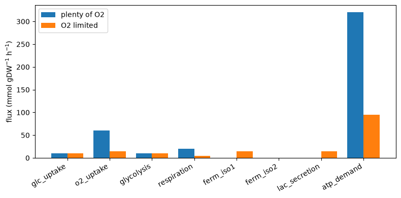
Alternate Optima and Flux Variability Analysis
A subtlety hides in the solution above: linprog returned one optimal flux distribution, but it is not the only one. Any split of the fermentation flux between the two isozymes and gives exactly the same ATP production. The optimal value of an LP is unique, but the optimal solution often is not — and at genome scale, with thousands of parallel routes, degeneracy is the rule rather than the exception. Interpreting a single arbitrary optimum as “the” predicted flux state is a common mistake.
Flux variability analysis (FVA) quantifies the degeneracy. For each reaction , it solves two additional LPs — minimize and maximize — while constraining the original objective to stay at its optimal value :
The resulting interval tells us how well determined each flux is at the optimum:
def fva(bounds, c):
    _, z_opt = fba(bounds, c)
    # pin the objective at its optimum via an extra equality constraint
    A_eq = np.vstack([S, c])
    b_eq = np.append(np.zeros(len(metabolites)), z_opt)
    ranges = []
    for i in range(len(reactions)):
        e = np.zeros(len(reactions)); e[i] = 1.0
        lo = linprog(e, A_eq=A_eq, b_eq=b_eq, bounds=bounds, method="highs")
        hi = linprog(-e, A_eq=A_eq, b_eq=b_eq, bounds=bounds, method="highs")
        ranges.append((lo.fun, -hi.fun))
    return pd.DataFrame(ranges, index=reactions, columns=["min", "max"])

print(fva(make_bounds(o2_max=15.0), objective).round(2))
min max
glc_uptake 10.0 10.0
o2_uptake 15.0 15.0
glycolysis 10.0 10.0
respiration 5.0 5.0
ferm_iso1 0.0 15.0
ferm_iso2 0.0 15.0
lac_secretion 15.0 15.0
atp_demand 95.0 95.0
Only the isozyme fluxes are undetermined: each can range between 0 and 15, so the model can say that 15 units of pyruvate must be fermented, but not which enzyme carries the flux. In real applications FVA is used to classify reactions as essential (flux always nonzero at the optimum), optional (range includes zero) or blocked (flux zero in every feasible solution), and to compare the metabolic capabilities of, say, different gut bacteria under a shared diet.
A related refinement is parsimonious FBA (pFBA): among all flux distributions achieving the optimal objective, pick one minimizing the total flux . The rationale is that flux costs enzyme, and enzyme costs resources — so of two equally productive states, the cell prefers the more economical one. pFBA removes wasteful loops from the reported solution (though it cannot break ties between exactly symmetric isozymes, as FVA just showed us).
Predicting Knockouts: Gene Essentiality
Because a GEM links genes to reactions through its GPR rules, we can simulate genetics. To knock out a gene in silico, we disable every reaction whose GPR rule evaluates to false without that gene — an and rule loses its reaction when any member is deleted, an or rule only when all isozymes are gone. Then we re-run FBA and compare the optimal objective with and without the gene:
for some cutoff . With only a complete loss of the objective counts. Knockout screens record whether a mutant grows at all, so cutoffs of a few percent of the wild-type objective are typical for essentiality (the next chapter uses 5%); a larger cutoff, such as the we use below, instead flags genes whose loss strongly impairs the cell.
In our toy model, let glycolysis be catalyzed by gene , respiration by the complex and , and the two fermentation isozymes by and :
gpr = {
    "glycolysis": "G1",
    "respiration": "G2 and G3",
    "ferm_iso1": "G4",
    "ferm_iso2": "G5",
}
genes = ["G1", "G2", "G3", "G4", "G5"]

def knockout_bounds(bounds, ko_gene):
    """Disable all reactions whose GPR rule fails without ko_gene."""
    bounds = list(bounds)
    state = {g: (g != ko_gene) for g in genes}
    for rxn, rule in gpr.items():
        if not eval(rule, {}, state):
            bounds[reactions.index(rxn)] = (0.0, 0.0)
    return bounds

bounds = make_bounds(o2_max=15.0)
_, z_wt = fba(bounds, objective)

rows = []
for g in genes:
    _, z_ko = fba(knockout_bounds(bounds, g), objective)
    rows.append({"knockout": g, "ATP": z_ko, "ratio": z_ko / z_wt,
                 "essential (cutoff 0.5)": z_ko / z_wt <= 0.5})
print(pd.DataFrame(rows).round(2).to_string(index=False))
knockout ATP ratio essential (cutoff 0.5)
G1 0.0 0.00 True
G2 20.0 0.21 True
G3 20.0 0.21 True
G4 95.0 1.00 False
G5 95.0 1.00 False
The simulation reproduces classical genetic logic. Deleting abolishes ATP production entirely — glycolysis is unconditionally essential. Deleting either subunit of the respiratory complex ( or ) drops the objective to 20/95 ≈ 21% of wild type — essential under our cutoff of 0.5 but not under a cutoff of a few percent, since the cell survives on fermentation alone. The isozymes and are individually dispensable, because the or redundancy lets the other one take over; only the double knockout would matter. Note also that essentiality is conditional: with unlimited oxygen, the fermentation genes would be irrelevant and respiration would dominate — an essential gene is essential for a given objective in a given environment.
This simple loop, scaled up to genome size, is one of the most successful uses of GEMs: predicted essentiality agrees with experimental knockout screens for roughly 90% of genes in E. coli and yeast. This figure comes from carefully curated models of two of the best-studied organisms there are, and, because most genes are non-essential, an agreement of this kind flatters the models; the next chapter looks at both points. Applications include finding drug targets (genes essential in a pathogen or a tumor model but dispensable in the host model), designing minimal genomes, and metabolic engineering — methods such as OptKnock search for knockout combinations that couple growth to the secretion of a desired product, so that evolution pushes production up rather than down. These design problems ask discrete questions (which reactions to remove?) and are formulated as mixed-integer linear programs — still solvable, if more expensive than plain LP.
From Toy Models to Genome Scale
Everything we did above transfers directly to real models; only the bookkeeping grows. Curated reconstructions like iML1515 or Human-GEM take years of manual work; for other organisms, draft models can be built automatically from the genome, as the next chapter describes. Nobody builds by hand: models are distributed in the standard SBML format and analyzed with toolboxes such as COBRApy in Python, which provides model.optimize(), flux_variability_analysis() and single_gene_deletion() as one-liners, or RAVEN in MATLAB.
Two extensions are particularly important for human data science:
Context-specific models. The generic human GEM describes what any human cell could do, but a hepatocyte and a neuron express different enzyme repertoires. By overlaying transcriptomics (or proteomics) on the GPR rules, algorithms such as tINIT extract the subnetwork actually available to a given cell type or patient sample, yielding cell-type- and even patient-specific models. This is the sense in which GEMs serve as an integration platform for omics data: the model supplies the mechanistic scaffold, the omics data selects the active parts. Personalized cancer models built this way have been used to find tumor-specific essential genes as candidate drug targets, and liver models of metabolic dysfunction-associated steatotic liver disease (MASLD, formerly called non-alcoholic fatty liver disease) correctly predicted altered demand for serine and glycine in patients — a hypothesis subsequently tested by supplementation studies.
Better constraints. Plain FBA constrains only stoichiometry and uptake bounds; its modern descendants add further physics. Enzyme-constrained models (e.g. the GECKO framework) include the enzymes themselves in the stoichiometry, using so that fluxes are limited by proteome capacity — with such constraints, overflow metabolism emerges without the oxygen cap that our toy model needed. Other variants integrate quantitative metabolomics to relax the steady-state assumption where measurements show metabolite levels changing.
For a deeper treatment, the primer What is flux balance analysis? by Orth et al. is the canonical starting point; O’Brien et al. review the broader family of constraint-based methods; and Gu et al. and Zhang & Hua survey applications in biotechnology and systems medicine.
Discussion Questions
The pseudo-steady state assumption sets for internal metabolites. What biological situations violate it, and what do we gain in exchange for accepting it?
Why are growth (biomass) and ATP production reasonable objective functions, while maximizing glucose uptake is not? What objective would you propose for a neuron, or for a liver cell exporting glucose during fasting?
In the FVA output, the two isozyme fluxes each ranged over . Does this mean either range endpoint is biologically plausible? What extra information would pin the split down?
Our knockout of the respiration complex left 21% of ATP production. Would you call it essential? Discuss how the essentiality cutoff trades false positives against false negatives, e.g. when nominating drug targets.
A metabolic network diagram (topology only) and a GEM (with stoichiometry) both contain glycolysis. Give a concrete question the GEM can answer that the diagram cannot.
What you should know after reading this chapter
You should be able to:
Describe the three layers of a genome-scale metabolic model (GEM): mass-balanced reactions, gene-protein-reaction (GPR) rules, and bounds with exchange reactions. Explain what its stoichiometry adds compared with a pathway diagram that records only topology.
Write down the stoichiometric matrix of a small reaction network, with one row per metabolite and one column per reaction, negative entries for consumed and positive entries for produced metabolites.
Explain the pseudo-steady-state assumption , why it removes the need for kinetic parameters, and why it leaves a whole space of feasible flux distributions rather than a single solution.
Write down FBA as a linear program, maximizing subject to and . Argue for a suitable objective, such as biomass or ATP production, and explain why maximizing a nutrient uptake is not meaningful.
Calculate the optimal fluxes of the toy model by hand, with unlimited and with capped oxygen uptake, and explain how the result reproduces overflow metabolism and the Warburg effect.
Explain why an FBA optimum is often not unique, and interpret the flux ranges from flux variability analysis (FVA).
Identify which reactions a gene knockout disables from the GPR rules (
andfor enzyme complexes,orfor isozymes), and judge whether the gene is essential with the criterion .
- Orth, J. D., Thiele, I., & Palsson, B. Ø. (2010). What is flux balance analysis? Nature Biotechnology, 28(3), 245–248. 10.1038/nbt.1614
- Brunk, E., Sahoo, S., Zielinski, D. C., Altunkaya, A., Dräger, A., Mih, N., Gatto, F., Nilsson, A., Preciat Gonzalez, G. A., Aurich, M. K., Prlić, A., Sastry, A., Danielsdottir, A. D., Heinken, A., Noronha, A., Rose, P. W., Burley, S. K., Fleming, R. M. T., Nielsen, J., … Palsson, B. O. (2018). Recon3D enables a three-dimensional view of gene variation in human metabolism. Nature Biotechnology, 36(3), 272–281. 10.1038/nbt.4072
- Burgard, A. P., Pharkya, P., & Maranas, C. D. (2003). Optknock: A bilevel programming framework for identifying gene knockout strategies for microbial strain optimization. Biotechnology and Bioengineering, 84(6), 647–657. 10.1002/bit.10803
- O’Brien, E. J., Monk, J. M., & Palsson, B. O. (2015). Using Genome-scale Models to Predict Biological Capabilities. Cell, 161(5), 971–987. 10.1016/j.cell.2015.05.019
- Gu, C., Kim, G. B., Kim, W. J., Kim, H. U., & Lee, S. Y. (2019). Current status and applications of genome-scale metabolic models. Genome Biology, 20(1). 10.1186/s13059-019-1730-3
- Zhang, C., & Hua, Q. (2016). Applications of Genome-Scale Metabolic Models in Biotechnology and Systems Medicine. Frontiers in Physiology, 6. 10.3389/fphys.2015.00413