2. Representations of pairwise alignments#
Before delving into the intricacies of the alignment algorithms, it’s crucial to understand the matrix representation of alignments. This approach is not just a computational convenience but a fundamental framework that encapsulates the complexity of aligning biological sequences. Here’s an overview of why matrices are used in sequence alignment and the significance of the traceback process.
2.1. Understanding Matrix Representation in Sequence Alignments#
2.1.1. The Essence of Matrices in Alignments#
Aligning sequences involves comparing each character of one sequence with every character of another to identify regions of similarity or difference. Given the combinatorial explosion of possible alignments with even moderate-length sequences, a brute-force approach to comparison is computationally infeasible. This is where matrices come into play, offering a structured and efficient way to represent all possible alignments between two sequences.
2.1.2. How Matrices Facilitate Alignment#
A matrix for sequence alignment is essentially a grid. Each cell in this grid represents a comparison point between a character from one sequence and another from the second sequence. Each cell of the matrix corresponds to the characters in the two sequences being aligned. And a path from the top left cell to the bottom right cell of the matrix represents a global alignment.
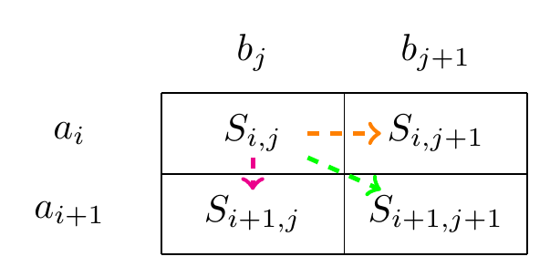
Fig. 2.1 A step in the path representing an alignment.#
If your alignment is in position \(a_i,b_j\) of two sequences \(\mathbf{a}=(a_1,\ldots,a_N)\) and \(\mathbf{b}=(b_1,\ldots,b_N)\) then the next step in the alignment is either a match/mismatch between \(a_{i+1},b_{j+1}\) (diagonal movement), a delete \(a_{i+1},-\), (a vertical movement), or an insert \(-,b_{j+1}\), (a horizontal movement).
2.1.3. Alignments as paths between the cells#
The path we follow tells us how the sequences should be aligned. A move diagonally signifies a match or mismatch, indicating that the characters from both sequences should be aligned with each other. Moving up or to the left indicates a gap in one of the sequences.
2.1.4. Examples of alignments#
An example of some matrix representations of an alignment is found in Fig. 2.2.
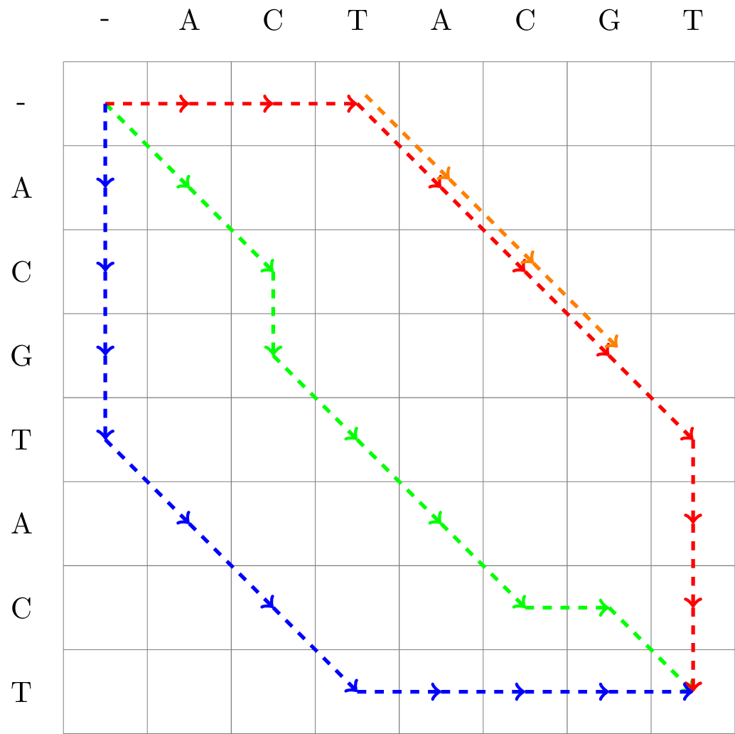
Fig. 2.2 Matrix representation of three full length alignments of ACGTACT and ACTACGT, as well as one partial alignment of the same sequences.#
The path of Alignment 1 is given in red, Alignment 2 in green, and Alignment 3 in blue. We also included a partial (local) alignment, Alignment 4 in orange.
Alignment 1 (red) |
Alignment 2 (green) |
Alignment 3 (blue) |
Alignment 4 (orange) |
|---|---|---|---|
|
|
|
|
|
|
|
|
The matrix representation of alignments and the traceback process are not merely computational techniques; they are integral to understanding the relationships between biological sequences. By breaking down the alignment process into a series of quantifiable steps, matrices allow us to systematically explore the vast space of alignment possibilities, leading us to the optimal alignment that best reflects the evolutionary or functional relationship between the sequences involved.
2.1.5. Exercises#
Exercise 2.1 (Matrix Representations of Alignments)
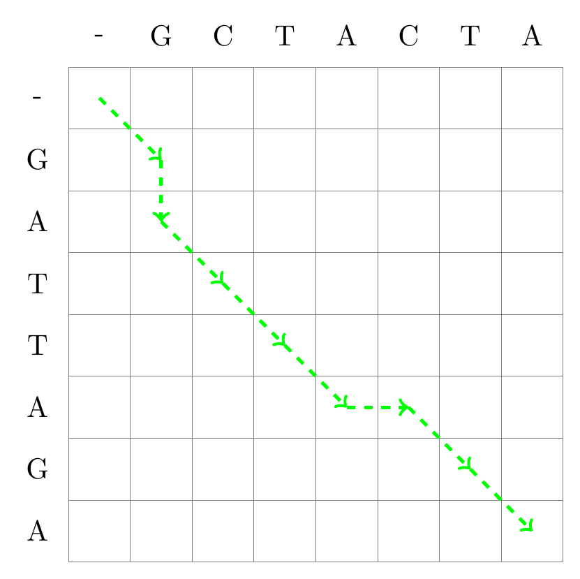
Which alignment does the following path represent?
Reveal Answer
GATTA-GA
G-CTACTA
2.2. Why Matrix Representations Are Useful#
Matrices are more than just a convenient way to visualize alignments — they form the mathematical foundation that allows us to apply efficient algorithms. The key property that makes them powerful is that they provide a structured way to exploit the principle of optimal substructure.
2.2.1. Optimal Substructure in Alignments#
When aligning two sequences, the score of the best alignment up to a given position \((i,j)\) depends only on:
the characters \(a_i\) and \(b_j\), and
the best scores of alignments leading into that position (from \((i-1,j-1)\), \((i-1,j)\), or \((i,j-1)\)).
This means that once we have computed the optimal score up to \((i,j)\), we no longer need to remember how we reached that point. The matrix cell itself summarizes all relevant information about the past.
In other words, any optimal scoring pathway of the subsequent part of the alignment is independent of the specific choices made earlier. This independence allows us to build solutions incrementally, storing partial results in the matrix and avoiding redundant computations.